hjic.mk.uni-pannon.hu DOI: 10.33927/hjic-2019-08
SIMULATION OF A BALANCED LOW-VOLTAGE ELECTRICAL GRID US- ING A SIMPLIFIED NETWORK MODEL
MÁRTONGREBER*1ANDATTILAFODOR1
1Department of Electrical Engineering and Information Systems, Faculty of Information Technology, University of Pannonia, Egyetem u. 10., Veszprém, H-8200, HUNGARY
A simulation method for low-voltage balanced distribution networks is proposed in this article. The novel method of node powers is based on the general calculation technique of node voltages. By researching only balanced networks, single- phase equivalents of the three-phase system are applicable. For the description of power lines, various parameters and matrices are available. In this work a simplified model is applied by using a purely resistive one. The active power results are solved through an iterative process. A main accomplishment is that the number of iterations needed is independent of the size of the network, and the process rapidly converges. Validation of the method is performed on the IEEE European Low-Voltage Test Feeder network. The simulation results confirm the achievements described in this paper.
Keywords: low-voltage distribution system, grid simulation, smart grid, method of node voltages, IEEE European Low-Voltage Test Feeder
1. Introduction
In recent years a lot of research has been conducted and progress made in the field of smart grid applications.
Therefore, the demand for cloud-based systems with in- tegrated simulation capabilities has increased. The calcu- lation of the voltages, currents and powers of the compo- nents of the electrical (smart) grid is not easily achieved.
This has resulted in the development of custom calcula- tion methods which have the benefit of being fine-tuned for a particular application.
One of the fundamental network calculation methods - in a general sense - is the node voltages method. From a mathematical perspective, this method is based on solv- ing a system of linear equations. As a result, this method can be implemented through various frameworks. One proposed solution revolves around using an open source discrete event simulator called OMNeT++ [1]. The mod- els for electrical components need to be constructeda and the simulation is conducted via message handling. An- other approach used Coloured Petri nets to model elec- trical networks [2]. A network model needs to be con- structed for the simulation, which consists of a propaga- tion process. A solution is presented for basic network types, while complex ones are calculated through decom- position. Both of these methods offer solutions but the method of node voltages regards currents as an input.
The more common approach to calculations of dis- tribution systems calculation is via the method of power
*Correspondence:greber.marton@virt.uni-pannon.hu
flow. This uses complex numbers to distinguish between active and reactive power. For the given nodes, both ac- tive and reactive power, voltage and phase angle are re- quired to formulate the solution [3]. This poses a non- linear problem, furthermore, the system of equations con- sists of real and imaginary subsets. Over the years, sev- eral pieces of research have dealt with this subject and the method known as DC power flow developed. By restrict- ing the parameters the calculation was simplified, namely the voltage angles as well as generated and consumed ac- tive powers. This method assumes small differences in voltage angle and lossless lines [4]. The biggest down- side of the method is that it cannot be used to calculate line losses because of the assumptions, although efforts are being made to overcome this obstacle [5].
By taking into account the extent of a given power system, different parameters of the power line model be- come dominant [6]. In low-voltage systems the distance between adjacent nodes is smaller than in high-voltage systems. By using this information a new set of restric- tions is proposed, inspired by the DC power flow. It can be regarded as a complementary method since the line re- actances are neglected. Utilising a resistive transmission line model offers the possibility to calculate distribution losses. This method has been developed from the method of node voltages.
In this article the issues of harmonic currents [7] and unbalanced networks [8] are not examined, it is assumed that the currents as well as voltages are sinusoidal and the grid is balanced with balanced three-phase loads. The
R7 Uv7
φ3
R5 φ2
R2 φ1
R1
Uv1
φ0
Ia4
R3
Uv6
R6
Figure 1:Example network
neutral wire can be omitted by restricting the set of net- works in balanced low-voltage systems. This enables the application of a one-line equivalent circuit.
2. Method of node voltages
In distribution network calculations the main emphasis is on power flow. That means the voltages and angles are calculable when the generated and consumed powers are given [9]. The known formula for calculating the active power in a DC network is the following:
P =U I, (1)
but the observed systems operate on alternating currents, hence the notion of AC power needs to be introduced [10]. Since voltages and currents are time-varying quanti- ties, these are expressed as complex numbers, namelyU andI. The complex power is calculated by multiplying the conjugate ofIby the voltage
S=U I∗. (2)
The phase angle of the complex power is defined by the difference between the angles of voltage and current:
ϕ= arg(U)−arg(I). (3) By observing the real and imaginary parts of the com- plex number, the active (P) and reactive powers (Q) are obtained:
P =Re(S), Q=Im(S). (4)
A known method for the analysis of electrical net- works is the method of node voltages. The component values, e.g. the sources of resistance, voltage and current are given, the unknown variables are the node voltages.
The calculation steps are best explained through an ex- ample network as shown inFig. 1.
One key component of the process is the definition of a directed graph for the example network shown in Fig. 2. The reference directions in the graph are arbitrary.
φ1 φ2 φ3
φ0
2
7
5
1
4 6 3
Figure 2:The reference directed graph
By using the graph in addition to Kirchoff’s first law, the nodal equations can be written in the following form:
I1−I2−I7= 0 I2−I3+I4+I5= 0 I7−I5+I6= 0
(5) After that, Ohm’s law is used to express the edge currents with regard to the nodal voltages:
I1=−G1(φ1−Uv1) I2=G2(φ1−φ2) I3=G3φ2 I4=Ia4
I5=G5(φ3−φ2) I6=−G6(φ3+Uv6) I7=G7(φ1+Uv7−φ3)
(6)
where the conductance of the arm of the network is de- noted by G. If these steps are followed, the system of equations must be rearranged. The final form can be ob- tained by substituting the currents intoEq.(5) and rear- ranging it to determine the nodal voltages [11]:
φ=G−1e Ie (7) The notation represents the dimensions of the elements it contains: the node voltage vector is obviously denoted by φ, the nodal admittance matrix byGeand the excitation vector byIe. At first sight, this equation does not account for the voltage sources in the branches. Since these ele- ments can be described in terms of current dimensions, the excitation vector takes the following form:
Ie=
−G1Uv1+G7Uv7
−Ia4
−G7Uv7+G6Uv6
. (8)
2.1 The generalized nodal equations
The above-mentioned method describes the working principle of the technique, but it is not suitable for algo- rithmic applications. A generalized approach is needed.
One has to define column vectors for the voltage sources:
Uv> =
uv1 uv2 . . . uvn
, (9)
current sources:
Ia>=
ia1 ia2 . . . ian
, (10)
and admittances:
Y>=
y1 y2 . . . yn
, (11)
whereY refers to the complex conductance known as the admittance. Each scalar of the vectors contains the afore- mentioned properties of a particular edge. For the repre- sentation of the graph, an incidence matrix (A) is used of(m−1)×ndimensions, and describes connections between nodes and edges:
ai,j=
0, ifjis not connected toi 1, ifjis pointing away fromi
−1, ifjis pointing towardsi
, (12)
wherei = 1,2, . . . , m−1 represents the nodes of the graph and j = 1,2, . . . , n denotes the edge index set.
As with the direction of the graph, the reference ofAis also arbitrary, it is only manifested when multiplied by (−1). These matrices can be constructed algorithmically and facilitate the use of the following equation [12]:
φ=YA−1A diag(Y)Uv−Ia
, (13)
where:
YA=Adiag(Y)A>. (14) A method which can be used to compute node voltages by defining a graph represented by the incidence matrix that includes the electrical properties of the edges is proposed as a result.
3. Network model
In order to reduce the amount of computational power that is needed for simulations, a simplified network model is used. The feeder points of low-voltage grids are trans- former substations which convert forward the desired power from the medium voltage side into the base volt- age, therefore, can be represented as voltage sources.
Power flows from the feeder points to the customers via transmission lines. Compared to medium- or high-voltage lines, the length between consecutive nodes is smaller. As a result, these can be modelled as series resistances. Cus- tomers are represented as current sources with consumer references of course.
The computationally demanding part of the method of node voltages is to invertYA. In the case of complex analyses, the system of equations is separated into real and imaginary parts. Through one iteration cycle, two in- verse calculations are needed. If voltages and currents are calculated as root mean square (RMS) values, the simu- lation method only requires real numbers. Therefore, the effort and time to calculate one cycle is halved.
2. Bus 3 Phase
10-35kV/0.4kV 1. Bus
3. Bus
4. Bus
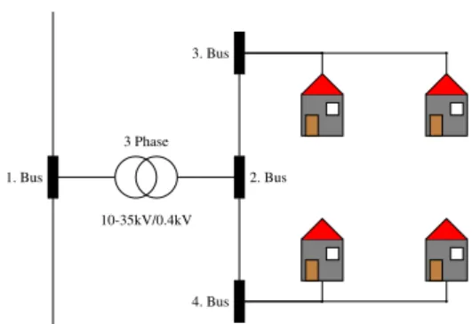
Figure 3:Low-voltage distribution system
3.1 Topology verification
In the structure of a low-voltage distribution network, some rules are noticeable. The transmission line forms a power rail to which the consumers can connect, as is shown inFig. 3. These mainly consist of households with single-phase connections, i.e. one phase and the neutral wire are used [13].
The method of node voltages can be applied to gen- eral circuits, on the other hand, the proposed method of node powers can be applied to distribution networks.
These form a tighter set, therefore, the topology needs to be checked to ensure it works properly.
If a network containsmnodes,mnode equations can be obtained. On the other hand, onlym−1equations are linearly independent. Therefore, one node can be omitted, namely the0V node is omitted in the proposed methods.
If an edge is connected to this point, it will have a non- zero column sum. If it is not connected to this point, it will have a column sum of zero. Using this, the criteria for the validation of topology can be formulated. The column sum for an arbitrary edge containing a current source in Acannot be equal to zero:
∀iaj6= 0, j∈ {1, . . . , n} →
m−1
X
i=1
ai,j 6= 0. (15)
Similarly, the column sum for an arbitrary edge contain- ing a voltage source inAcannot be equal to zero:
∀uvj 6= 0, j∈ {1, . . . , n} →
m−1
X
i=1
ai,j6= 0. (16)
In the case of an edge that possesses admittance, the col- umn sum inAmust be zero:
∀yj6= 0, j∈ {1, . . . , n} →
m−1
X
i=1
ai,j = 0. (17)
InAlgorithm 1, a pseudo code is shown that implements the above-mentioned criteria. It returns a Boolean value and is only true if the network topology is appropriate.
Algorithm 1Topology verification INPUT:A,Y,Ia,Uv
OUTPUT:IsValidTopology
1: IsValidTopology= 1
2: n=NumberOfColumns(A)
3: fori= 1tondo
4: s= 0
5: ifIa(i) ! = 0then
6: s= sum(A(:, i))
7: ifs== 0then
8: IsValidTopology= 0
9: end if
10: end if
11: ifUv(i) ! = 0then
12: s= sum(A(:, i))
13: ifs== 0then
14: IsValidTopology= 0
15: end if
16: end if
17: ifY(i) ! = 0then
18: s= sum(A(:, i))
19: ifs! = 0then
20: IsValidTopology= 0
21: end if
22: end if
23: end for
4. Method of node powers
Since the simulated households are single-phase con- sumers, the corresponding active power can be calculated as follows:
P=U I cos(ϕ). (18) Let us define the power factor (PF) and current-source active power (Pa) vectors for further matrix calculations.
Single elements in both of these describe properties with regard to a single edge.
PF>=
cos(ϕ1) cos(ϕ2) . . . cos(ϕn) , (19) Pa>=
pa1 pa2 . . . pan
. (20)
Voltage can be expressed as the electric potential differ- ence between two points. If the incidence matrix rep- resents node-edge relations, transposing it will describe edge-node relations. Multiplying it with the node volt- ages column vector will result in edge voltages:
U =A>φ. (21) By determining these notations and definitions, the basic equation of node voltage can be extended:
φ=YA−1A diag(Y)Uv−Ia Pa= diag(PF)diag(A>φ)Ia
, (22) In the case of the method of node voltages, the node voltages are calculated using the given current consump- tion. However, in the case of the method of node powers,
the node voltages must be calculated with regard to the consumption, given in terms of the active power.Eq. 22 opens up the possibility of finding a solution following a trial and error procedure.
In other words, if only one current source in this sys- tem of equations is changed, all the node voltages will also be changed. Let us consider the case where the cur- rent of one particular customer is changed until its active power becomes equal to its actual value. Nonetheless, if a second consumer is to be set in the same fashion, the first one will be ruined. Through positive changes in current to the second source, a net drop in voltage will occur. Since power is the product of current and voltage, the current was untouched so the active power will be less. There- fore, it is also clear that if the second current source is decreased, the active power of the first source will exceed its actual value.
4.1 Constant iteration current
In the aforementioned problem, the solution is acquired through an iterative process to build up the unknown cur- rents of the system gradually, instead of trying to deter- mine them individually. It is necessary to choose a value of the current for the iterations:Iiter. In the first step, ev- ery element of the current vector is zero, however, if an edge contains a consumer, its value will be set as the iter- ation current. The problem, namely that by changing one current, all the node voltages will also change, still ex- ists. However, if the iteration current is sufficiently small, the ability to build up the parameters from the ground is viable. To select a source for the actual iteration, a new variable was defined:
dPP = Pasim Pa
. (23)
This can be calculated for all consumer edges per itera- tion and provides information about how similar the sim- ulated active power is to its desired value. It is obvious that the edge with the smallestdPP requires the highest degree of correction, therefore, it is incremented byIiter. Consequently, in every iteration the branch with the min- imumdPP needs to be identified, using a simple mini- mum search. After appropriate incrementation, the node voltages must be calculated in order to determine the new values of power. This procedure can be observed inAl- gorithm 2.
In an ideal case, the algorithm converges into the de- sired power vector and the following expression will be true:
∀i∈ {1, . . . , k} →dPPi= 1, (24) wherekdenotes the number of consumers in the grid. It is clear that the rate of convergence and the accuracy of the algorithm are heavily influenced byIiter. If this rate is particularly small, the results will be precise (dPP = 1).
However, in this case the number of iteration cycles will be enormous because the function described is analogous
Algorithm 2Constant iteration current INPUT:A,Y,Pa,Uv,PF,Iiter,m,n OUTPUT:φ,Ia
1: Ia= zeros(n,1)
2: fori= 1tondo
3: ifPa(i) ! = 0then
4: Ia(i) =Iiter
5: end if
6: end for
7: φ= CalculateNodeVoltages(A,Y,Uv,Ia)
8: Pasim= diag(diag(A>·φ)·Ia)·PF
9: [dPP, index] = min(Pasim/Pa)
10: whiledPP < do
11: Ia(index) =Ia(index) +Iiter
12: φ= CalculateNodeVoltages(A,Y,Uv,Ia)
13: Pasim= diag(diag(A>·φ)·Ia)·PF
14: [dPP, index] = min(Pasim/Pa)
15: end while
to x1. This can be observed by determining the actual number of iterations needed for the process:
k
X
i=1
Iai Iiter
(25) as the desired current will consist of portions ofIiter on every edge. According to how the desired current is di- vided by the iteration current, overshoots are possible.
Therefore, a value ofis needed in order to secure a suit- able exit condition for the loop.
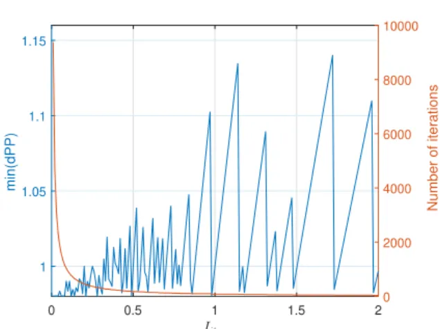
Basically the blue plot represents a function similar tof(x) =cmodx, wherecdenotes a given number. In the case of the method described,c stands for a desired load current andxrepresents possible iteration currents used in the algorithm. According to how the desired cur- rent is divided by the actual iteration current, false values can be calculated. The periodic increase in the error is a property of the modulo operation, since the remainder in- creases until an integer multiple ofxis identified. Then the error is equal to zero but begins to increase again.
The red line represents the number of iterations needed to converge into a final solution. Ifx << c, the maximum
"overshoot" by the modulo operator is relatively small, on the other hand, ifx < c, more significant errors can occur. It is clear that in the first case many more iterations are necessary than in the second. Sinceccannot be deter- mined beforehand, unnecessarily large errors can occur which represents the weakness of the algorithm.
It is clear that a compromise must be made between the run-time and precision, as illustrated inFig. 4.
4.2 Dynamic iteration current
To fix the weaknesses of the algorithm elaborated on in the previous chapter, an advanced version was developed.
The first aspect, in which there is room for improvement, is to obtain reasonable initial values ofIa. The process
0 0.5 1 1.5 2
Iiter 1
1.05 1.1 1.15
min(dPP)
0 2000 4000 6000 8000 10000
Number of iterations
Figure 4:Minimum error - number of iterations
does not have to originate fromIai = 0, consequently, a considerable amount of cycles can be skipped. In distri- bution networks the deviation from the nominal voltage (Un) is always regulated by standards, for example, in Hungary it is approximately±7.5%. Using this restric- tion, a general estimation can be made for the nodes. The followingmin()andmax() operators relate to the val- ues of the given function. The possible interval between current values can be formulated as follows:
min(Ia) = pai Uncos(ϕi) max(Ia) = pai
(1−D)Uncos(ϕi)
, (26)
where D is the aforementioned deviation value. This means overestimating the voltage results in the minimum value of the current. Setting the starting values of the cur- rents according to the minimum approximation is ade- quate. To calculate the maximal remaining error, the min- imum value ofdPPineeds to be calculated:
dPPi=
Un(1−D)U pai
ncos(ϕi)cos(ϕi) pai
= 1−D. (27) The logic behind this equation is as follows: the fraction in the numerator is the minimum current estimation the Un(1−D), on the other hand, is the worst case scenario in terms of the voltage. The deviation is defined by D, so under no circumstances can the voltage drop below Un(1−D), once the initial value has been set. Because Dis small, this approach alone solves a huge part of the problem, since by taking the Hungarian voltage levels as an example, a dPP value greater or equal to 0.925 is achieved!
Since the initial value problem has been solved, the remaining iterations can also be improved by taking the aforementioned method one step further. In order to take the absolute error in the active power into account, the following variable is introduced:
dP =Pa−Pasim. (28)
which can also be formulated using the relative error:
dP =Pa(1−dPP). (29) Since the whole algorithm is founded on an iterative method, it would be suitable to use the minimum estima- tion process of the worst-case scenario in the following iterations. The idea in theory, however, is similar to the power value that is being approximated changes. Only the remaining error component needs to be recalculated.
Therefore, the approximation will take the givendPiinto consideration instead of the wholepai.Un can still be used for this, but is not ideal. Once the initial values are set, a node voltage calculation is performed, thus the new node voltages can be used. As a result, the new values must be used as the upper limit of the voltage. Finally, the current generated for a particular consumer can be represented by the following series:
Iai= 1 cos(ϕi)
pai Un
|{z}j=1
+dPi0 φ0i
|{z}j=2
+dPi00 φ00i
| {z }
j=3
+. . .
, (30)
wherej = 1,2, . . .denotes the number of iterations. If j → ∞, the simulated values approach the desired ac- tive powers. In theory this would mean that an infinite number of iterations would be necessary. The maximum error or minimumdPPcan be calculated as shown before not only for the initial values but also for the upcoming iteration currents. Since in every consequent cycle the ab- solute error from the previous cycle is corrected, the re- mainingdP will be corrected by a minimumdPP equal to(1−D). Since the fitted values are multiplied, the min- imum value of thej-th iteration can be calculated as fol- lows:
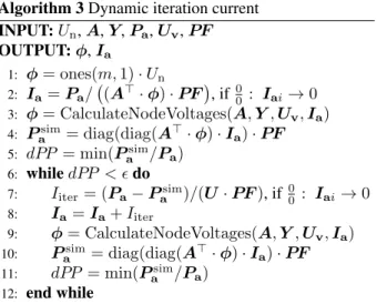
dPPmin= 1−Dj. (31) The process of the method of dynamic node pow- ers is shown inAlgorithm 3. In the literature review, the
Algorithm 3Dynamic iteration current INPUT:Un,A,Y,Pa,Uv,PF OUTPUT:φ,Ia
1: φ= ones(m,1)·Un 2: Ia=Pa/ (A>·φ)·PF
, if00 : Iai→0
3: φ= CalculateNodeVoltages(A,Y,Uv,Ia)
4: Pasim= diag(diag(A>·φ)·Ia)·PF
5: dPP= min(Pasim/Pa)
6: whiledPP < do
7: Iiter= (Pa−Pasim)/(U·PF), if00 : Iai →0
8: Ia=Ia+Iiter
9: φ= CalculateNodeVoltages(A,Y,Uv,Ia)
10: Pasim= diag(diag(A>·φ)·Ia)·PF
11: dPP = min(Pasim/Pa)
12: end while
Newton-Raphson method was examined in more detail which uses the mismatch in power by incorporating the Jacobian matrix in order to achieve convergence. The pro- posed error recalculation method was developed whilst taking that process into consideration. Another possible solution to the calculation of powers could be an algo- rithm, in which the total power is recalculated rather than the power mismatch. The explicit expression for conver- gence was determined first, and the total power recalcu- lation method did not suggest better results.
Although through simulation and observation, it was noted that both require the same amount of iterations. Us- ing the Monte Carlo method, a large number of random networks were created in order to monitor the run-time.
Results showed the presence of slight deviations with regard to each other. Nevertheless, the two methods re- quire almost the same amount of computational time, as is shown inFig. 5.
0 30 0.002 0.004
100 0.006
Runtime[s]
20 0.008
Error recalculation algorithm
Number of streets ~ Network size 0.01
Unique simulations 0.012
10 50 0 0
0 30 0.002 0.004
100 0.006
Runtime[s]
20 0.008
Whole power recalculation algorithm
Number of streets ~ Network size 0.01
Unique simulations 0.012
10 50 0 0
Figure 5:Monte Carlo simulation
Figure 6:The topology of the test network
5. Simulation results
In order to verify the proposed method properly, a ref- erence network with available simulation data was re- quired. For verification purposes the IEEE European Low-Voltage Test Feeder network [14] was used. The simulation process consisted of the implementation of the stated algorithm and importation of network data using MATLAB. The topology of the test grid is shown inFig.
6.
Some of the important network parameters are the fol- lowing: it consists of906nodes which are connected by 927edges that supply55single-phase consumers. Previ- ous runs have shown that approximately2iterations are sufficient for engineering purposes. For the sake of accu- racy, a limit was set fordPP, thereforeis still shown in Algorithm 3.
The minimum estimations ofdPP predicted that the error should rapidly converge to zero. The simulation ver- ified this statement, the rapid decrease in the absolute er- ror can be seen inTables 1 - 3. It can be clearly observed that in the case of a network of such a size, the maximum voltage difference can be maintained under10mV (Table 4).
The results of the simulation can be seen in Fig. 7 which represents the bus voltages of a single phase. Note that theyaxis is divided into increments of50mV.
Table 1:Convergence ofdPin Phase ‘A’
Iteration max (dP) 0. 0.052137599675W 1. 0.000041085202W 2. 0.000000032240W
Table 2:Convergence ofdPin Phase ‘B’
Iteration max (dP) 0. 0.042119472811W 1. 0.000029088116W 2. 0.000000019550W
Table 3:Convergence ofdPin Phase ‘C’
Iteration max (dP) 0. 0.043952897250W 1. 0.000025174297W 2. 0.000000014771W
Table 4:Maximum voltage differences Phase ‘A’ Phase ‘B’ Phase ‘C’
0.056859V 0.036058V 0.023649V
Since the active power values are reached with an ex- cellent degree of precision, one would expect that the voltage differences would be smaller. However, this ef- fect does not originate from the algorithm, rather from the simplified network model. This facilitates the possi- bility of achieving small simulation times. Since the in- troduction of the method of dynamic iteration currents, the number of iterations is independent of the size of the network. The computationally heavy component is the calculation of the inverse ofYA. The topology of the net- work remains unchanged during the iterations. Therefore, the steady state simulation of a three-phase network re- quires, independen of the network size, only three matrix inversions. The duration of the simulation of this network was2.29s at a particular instant.
0 100 200 300 400 500 600 700 800 900 1000
Bus ID 251.9
251.95 252 252.05 252.1 252.15 252.2
Voltage [V]
IEEE reference Simulation
Figure 7:Simulation results for phase ‘A’
6. Conclusion
A novel simulation method for low-voltage distribution networks is proposed in this paper. The existing method of node voltages is further developed in order to handle active power calculations in low-voltage grids. These sys- tems consist of a unique topology to which the process was fitted. The verification criteria for the network struc- ture was formulated. A solution was proposed in which the number of iterations is independent of the size of the network and the simulation error decreases exponentially.
The method was tested and verified on the IEEE Euro- pean Low-Voltage Test Feeder network. This confirmed the statements about the algorithm. Insignificant errors appeared in the test results but these were the effect of the simplified network model.
In the future, the algorithm could be improved to han- dle unbalanced distribution networks. With the aid of appropriate modifications, distributed generation could be taken into consideration that accounts for not only power consumption but also generation. The algorithm can serve as a foundation of network diagnostics by us- ing it to detect faults as well as technical or non-technical losses.
Acknowledgement
We acknowledge the financial support of Széchenyi 2020 under the EFOP-3.6.1-16-2016-00015. We acknowledge the financial support of Széchenyi 2020 under the GINOP-2.2.1-15-2017-00038.
Notations
φ Node-voltage vector Ie Excitation vector Uv Voltage-source vector Ia Current-source vector A Incidence matrix Y Admittance matrix YA Nodal admittance matrix m Number of nodes n Number of edges cos(ϕ) Power factor PF Power factor vector
Pa Current-source active-power vector U Branch voltage vector
dPP Delta power percentage Iiter Iteration current dP Delta power
D Voltage level deviation Pasim Simulated power vector
S Complex power
P Active power
Q Reactive power
ϕ Phase angle
G Conductance
Threshold value for iteration
REFERENCES
[1] S˝orés, M.; Fodor, A.: Simulation of electrical grid with OMNeT++ open source discrete event system simulator,Hung. J. Ind. Chem., 201644(2), 85–91,
DOI: 10.1515/hjic-2016-0010
[2] Pózna, A.I.; Fodor, A.; Gerzson, M.; Hangos, K.M.:
Colored Petri net model of electrical networks for diagnostic purposes,IFAC-PapersOnLine, 2018 51(2), 260–265,DOI: 10.1016/j.ifacol.2018.03.045
[3] Stagg, G.; El-Abiad, A.H.: Computer methods in power system analysis (McGraw-Hill), intern- taional student edn., 1968
[4] Hertem, D.V.; Verboomen, J.; Purchala, K.; Bel- mans, R.; Kling, W.L.: Usefulness of DC power flow for active power flow analysis,The 8th IEE International Conference on AC and DC Power Transmission, 20061,DOI: 10.1049/cp:20060013
[5] Stott, B.; Jardim, J.; Alsac, O.: DC power flow revis- ited,IEEE T. Power Syst., 200924(3), 1290–1300,
DOI: 10.1109/TPWRS.2009.2021235
[6] Das, J.C.: Load flow optimazitaion and optimal power flow (CRC Press), 2017
[7] Görbe, P.; Magyar, A.; Hangos, K.M.: THD re- duction with grid synchronized inverter’s power in- jection of renewable sources, in 2010 International Symposium on Power Electronics Electrical Drives Automation and Motion (SPEEDAM) (IEEE), 1381–1386,DOI: 10.1109/SPEEDAM.2010.5545079
[8] Neukirchner, L.; Görbe, P.; Magyar, A.: Voltage un- balance reduction in the domestic distribution area using asymmetric inverters,J. Clean. Prod., 2017 142, 1710–1720,DOI: 10.1109/59.575728
[9] Kersting, W.H.: Distribution system modeling and analysis (CRC Press), 2016,ISBN: 9781439856475
[10] Bird, J.: Electrical circuit theory and technology (Taylor & Francis), 4th edn., 2010,ISBN: 185617770X
[11] Wang, X.F.; Song, Y.; Irving, M.: Modern power system analysis (Springer), 2008,DOI: 10.1007/978-0- 387-72853-7
[12] Zhang, F.; Cheng, C.S.: A modified Newton method for radial distribution system power flow analysis, IEEE T. Power Syst., 199712(1), 389 – 397, DOI:
10.1109/59.575728
[13] Westinghouse Electric Corporation, Electrical transmission and distribution reference book (East Pittsburgh, PA), 1964
[14] Schneider, K.P.; Mather, B.A.; Pal, B.C.; Ten, C.W.; Shirek, G.J.; Zhu, H.; Fuller, J.C.; Pereira, J.L.R.; Ochoa, L.F.; de Araujo, L.R.; Dugan, R.C.;
Matthias, S.; Paudyal, S.; McDermott, T.E.; Ker- sting, W.: Analytic considerations and design ba- sis for the IEEE distribution test feeders, IEEE T.
Power Syst., 201733(3), 3181–3188,DOI: 10.1109/TP- WRS.2017.2760011