Performance Analysis of Sparse MatrixRepresentation in Hierarchical Temporal Memoryfor Sequence Modeling

(1)

Performance Analysis of Sparse Matrix Representation in Hierarchical Temporal Memory for Sequence Modeling

1 Balatonfüred Student Research Group

1,2Department of Telecommunications and Media Informatics, Budapest University of Technology and Economics Budapest, Hungary

3Numenta is a nonprofit research group dedicated to developing the Hierarchical Temporal Memory.

E-mail: csongor.pilinszkinagy@gmail.com; toth.b@tmit.bme.hu

INFOCOMMUNICATIONS JOURNAL

Performance Analysis of Sparse Matrix

Representation in Hierarchical Temporal Memory for Sequence Modeling

Csongor Pilinszki-Nagy¹and Bálint Gyires-Tóth²

Performance Analysis of Sparse Matrix

Representation in Hierarchical Temporal Memory for Sequence Modeling

Csongor Pilinszki-Nagy, B´alint Gyires-T´oth Department of Telecommunications and Media Informatics

Budapest University of Technology and Economics Budapest, Hungary

Email: csongor.pilinszkinagy@gmail.com, toth.b@tmit.bme.hu

Abstract—Hierarchical Temporal Memory (HTM) is a special type of artificial neural network (ANN), that differs from the widely used approaches. It is suited to efficiently model sequential data (including time series). The network implements a variable order sequence memory, it is trained by Hebbian learning and all of the network’s activations are binary and sparse. The network consists of four separable units. First, the encoder layer translates the numerical input into sparse binary vectors. The Spatial Pooler performs normalization and models the spatial features of the encoded input. The Temporal Memory is responsible for learning the Spatial Pooler’s normalized output sequence. Finally, the decoder takes the Temporal Memory’s outputs and translates it to the target. The connections in the network are also sparse, which requires prudent design and implementation. In this paper a sparse matrix implementation is elaborated, it is compared to the dense implementation. Furthermore, the HTM’s performance is evaluated in terms of accuracy, speed and memory complexity and compared to the deep neural network-based LSTM (Long Short-Term Memory).

Index Terms—neural network, Hierarchical Temporal Mem- ory, time series analysis, artificial intelligence, explainable AI, performance optimization

I. INTRODUCTION

Nowadays, data-driven artificial intelligence is the source of better and more flexible solutions for complex tasks compared to expert systems. Deep learning is one of the most focused research area, which utilizes artificial neural networks. The complexity and capability of these networks are increasing rapidly. However, these networks are still ’just’ black (or at the best grey) box approximators for nonlinear processes.

Artificial neural networks are loosely inspired by neurons and there are fundamental differences [1], that should be implemented to achieve Artificial General Intelligence (AGI), according to Numenta [2], [3].¹They are certain that AGI can only be achieved by mimicking the neocortex and implement- ing those fundamental differences in a new neural network model.

Artificial neural networks require massive amount of computational performance to train the models through many epochs. Also, the result of a neural network training is not,

or only partly understandable, it remains a black (or at best a grey) box system. There is a need to produce explainable AI solutions, that can be understood. Understanding and modeling the human brain should deliver a better understanding of the decisions of the neural networks.

Sequence learning is a domain of machine learning that aims to learn sequential and temporal data, and time series. Through the years there were several approaches to solve sequence learning. The state of the art deep learning solutions use one-dimensional convolutional neural networks [4], recurrent neural networks with LSTM type cells [5], [6] and dense layers with attention [7]. Despite the improvements over other solutions these algorithms still lack some of the preferable properties, that would make them ideal for sequence learning [1]. The HTM network utilizes a different approach.

Since the HTM network is sparse by nature, it is desirable to implement it in such a way that exploits the sparse structure.

Since other neural networks work using optimized matrix implementations, a sparse matrix version is a viable solution to that. This porting should be a two-step process: first a matrix implementation of the HTM network, then a transition to sparse variables inside the network. These ideas are partially present in other experiments, still, this approach remains a unique way of executing HTM training steps. Our goal is to realize and evaluate an end-to-end sparse solution of the HTM network, which utilizes optimized (in terms of memory and speed) sparse matrix operations.

The contributions of this paper are the following:

• Collection of present HTM solutions and their specifics

• Proposed matrix solution for the HTM network

• Proposed sparse matrix solution for the HTM network

• Evaluation of training times for every part of the HTM network

• Evaluation of training times compared to LSTM network

• Evaluation of training and testing accuracy compared to LSTM network

II. BACKGROUND

There have been a number of works on different sequence learning methods (e.g., Hidden Markov Models [8], Autore-

Performance Analysis of Sparse Matrix

Representation in Hierarchical Temporal Memory for Sequence Modeling

I. INTRODUCTION

II. BACKGROUND

Performance Analysis of Sparse Matrix

Representation in Hierarchical Temporal Memory for Sequence Modeling

I. INTRODUCTION

II. BACKGROUND

for Sequence Modeling

I. INTRODUCTION

II. BACKGROUND

Artificial neural networks are loosely inspired by neurons and there are fundamental differences [1], that should be implemented to achieve Artificial General Intelligence (AGI), according to Numenta [2], [3]. ³ They are certain that AGI can only be achieved by mimicking the neocortex and implement- ing those fundamental differences in a new neural network model.

Artificial neural networks require massive amount of computational performance to train the models through many

(2)

gressive Integrated Moving Average (ARIMA) [9]), however, in this paper artificial neural network-based solutions are investigated.

A. Deep learning-based sequence modeling

Artificial neural networks evolved in the last decades and were popularized again in the last years, thanks to the advances in accelerated computing, novel scientific methods and the vast amount of data. The premise of these models is the same: build a network using artificial neurons and weights, that are the nodes in layers and weights connecting them, correspondingly. Make predictions using the weights of the network, and backpropagate the error to optimize weight values based on a loss function. This iterative method can achieve outstanding results [10], [11].

Convolutional neural networks (CNN) utilize the spatial features of the input. This has great use for sequences, since it is able to find temporal relations between timesteps. This type of network works efficiently by using small kernels to execute convolutions on sequence values. The kernels combined with pooling and regularization layers proved to be a powerful way to extract information layer by layer from sequences [12], [4].

Recurrent neural networks (RNN) use previous hidden states and outputs besides the actual input for making predictions.

Baseline RNNs are able only to learn shorter sequences. The Long Short-Term Memory (LSTM) cell can store and retrieve the so called inner state and thus, it is able to model longer sequences [13]. Advances in RNNs, including hierarchical learning and attention mechanism, can deliver near state- of-the-art results [14], [15], [16]. An example of advanced solutions using LSTMs is the Hierarchical Attention Network (HAN) [17]. This type of network contains multiple layers of LSTM cells, which model the data on different scopes, and attention layers, which highlight the important parts of the representations.

Attention mechanism-based Transformer models achieved state-of-the-art results in many application scenarios [7]. How- ever, to outperform CNNs and RNNs, a massive amount of data and tremendous computational performance are required.

B. Hierarchical Temporal Memory

Hierarchical Temporal Memory (HTM) is a unique approach to artificial intelligence that is inspired from the neuroscience of the neocortex [1]. The neocortex is responsible for human intelligent behavior. The structure of the neocortex is homoge- neous and has a hierarchical structure where lower parts process the stimuli, and higher parts learn more general features.

The neocortex consists of neurons, segments, and synapses.

There are vertical connections that are the feedforward and feedback information between layers of cells and there are horizontal connections that are the context inputs. The neurons can connect to other nearby neurons through segments and synapses.

HTM is based on the core assumption that the neocortex stores and recalls sequences. These sequences are patterns of the Sparse Distributed Representation (SDR) input, which are

translated into the sequences of cell activations in the network.

This is an online training method, which doesn’t need multiple epochs of training. Most of the necessary synapse connections are created during the first pass, so it can be viewed as a one- shot learning capability. The HTM network can recognize and predict sequences with such robustness, that it does not suffer from the usual problems hindering the training of conventional neural networks. HTM builds a predictive model of the world, so every time it receives input, it is attempting to predict what is going to happen next. The HTM network can not only predict the future values of sequences but e.g., detect anomalies in sequences.

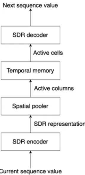
Fig. 1. HTM block diagram

The network consists of four components: SDR Encoder, Spatial Pooler, Temporal Memory, and SDR decoder (see Figure 1).

The four components do the following:

• The SDR Scalar Encoder receives the current input value and represent it an SDR. An SDR representation is a binary bit arrays that retains the semantic similarity between similar input values by overlapping bits.

• The Spatial Pooler activates the columns given the SDR representation of the input. The Spatial Pooler acts as a normalization layer for the SDR input, which makes sure the number of columns and the number of active columns stay fixed. It also acts as a convolutional layer by only connecting to specific parts of the input.

• The Temporal Memory receives input from the Spatial Pooler and does the sequence learning, which is expressed in a set of active cells. Both the active columns and active cells are sparse representations of data just as the SDRs.

These active cells not only represent the input data but provide a distinct representation about the context that came before the input.

• The Scalar Decoder takes the state of the Temporal Memory and treating it as an SDR decodes it back to scalar values.

1) Sparse Distributed Representation: The capacity of a dense bit array is 2 to the power of the number of bits. It is a large capacity coupled with low noise resistance.

Fig. 2. SDR matching

A spare representation bit array has smaller capacity but is more robust against noise. In this case the network has a 2% sparsity, which means, that only the 2% of columns are activated [1]. A sparse bit array can be stored efficiently by only storing the indices of the ones.

To enable classification and regression there needs to be a way to decide whether or not two SDRs are matching. An illustration for SDR matching can be found in Figure 2. If the overlapping bits in two SDRs are over the threshold, then it is considered as a match. The accidental overlaps in SDRs are rare so the matching of two SDRs can be done with high precision. The rate of a false positive SDR matching is meager.

2) Encoder and decoder: The HTM network works exclu- sively with SDR inputs. There needs to be an encoder for it so that it can be applied to real-world problems. The first and most critical encoder for the HTM system is the scalar encoder. Such an encoder for the HTM is visualized by the Figure 3

Fig. 3. SDR encoder visualization

The principles of SDR encoding:

• Semantically similar data should result in SDRs with overlapping bits. The higher the overlap, the more the similarity.

• The same input should always produce the same output, so it needs to be deterministic.

• The output should have the same dimensions for all inputs.

• The output should have similar sparsity for all inputs and should handle noise and subsampling.

The prediction is the task of the decoder, which takes an SDR input and outputs scalar values. This time the SDR input is the state of the network’s cells in the Temporal Memory. This part of the network is not well documented, the only source is the implementation of the NuPIC package [18]. The SDR decoder visualization is presented in Figure 4.

Fig. 4. SDR decoder visualization

3) Spatial Pooler: The Spatial Pooler is the first layer of the HTM network. It takes the SDR input from the encoder and outputs a set of active columns. These columns represent the recognition of the input and they compete for activation. There are two tasks for the Spatial Pooler, maintain a fixed sparsity and maintain overlap properties of the output of the encoder. These properties can be looked at like the normalization in other neural networks which helps the training process by constraining the behavior of the neurons.

The Spatial Pooler is shown in Figure 5

Fig. 5. Spatial Pooler visualization

The Spatial Pooler has connections between the SDR input cells and the Spatial Pooler columns. Every synapse is a potential synapse that can be connected or not depending on its strength. At initialization, there are only some cells connected to one column with a potential synapse. The randomly initialized Spatial Pooler already satisfies the two criteria, but a learning Spatial Pooler can do an even better representation of the input SDRs.

The activation is calculated from the number of active synapses for every column. Only the top 2% is allowed to be activated, the others are inhibited.

(3)

gressive Integrated Moving Average (ARIMA) [9]), however, in this paper artificial neural network-based solutions are investigated.

A. Deep learning-based sequence modeling

Artificial neural networks evolved in the last decades and were popularized again in the last years, thanks to the advances in accelerated computing, novel scientific methods and the vast amount of data. The premise of these models is the same: build a network using artificial neurons and weights, that are the nodes in layers and weights connecting them, correspondingly. Make predictions using the weights of the network, and backpropagate the error to optimize weight values based on a loss function. This iterative method can achieve outstanding results [10], [11].

Convolutional neural networks (CNN) utilize the spatial features of the input. This has great use for sequences, since it is able to find temporal relations between timesteps. This type of network works efficiently by using small kernels to execute convolutions on sequence values. The kernels combined with pooling and regularization layers proved to be a powerful way to extract information layer by layer from sequences [12], [4].

Recurrent neural networks (RNN) use previous hidden states and outputs besides the actual input for making predictions.

Baseline RNNs are able only to learn shorter sequences. The Long Short-Term Memory (LSTM) cell can store and retrieve the so called inner state and thus, it is able to model longer sequences [13]. Advances in RNNs, including hierarchical learning and attention mechanism, can deliver near state- of-the-art results [14], [15], [16]. An example of advanced solutions using LSTMs is the Hierarchical Attention Network (HAN) [17]. This type of network contains multiple layers of LSTM cells, which model the data on different scopes, and attention layers, which highlight the important parts of the representations.

Attention mechanism-based Transformer models achieved state-of-the-art results in many application scenarios [7]. How- ever, to outperform CNNs and RNNs, a massive amount of data and tremendous computational performance are required.

B. Hierarchical Temporal Memory

Hierarchical Temporal Memory (HTM) is a unique approach to artificial intelligence that is inspired from the neuroscience of the neocortex [1]. The neocortex is responsible for human intelligent behavior. The structure of the neocortex is homoge- neous and has a hierarchical structure where lower parts process the stimuli, and higher parts learn more general features.

The neocortex consists of neurons, segments, and synapses.

There are vertical connections that are the feedforward and feedback information between layers of cells and there are horizontal connections that are the context inputs. The neurons can connect to other nearby neurons through segments and synapses.

HTM is based on the core assumption that the neocortex stores and recalls sequences. These sequences are patterns of the Sparse Distributed Representation (SDR) input, which are

translated into the sequences of cell activations in the network.

This is an online training method, which doesn’t need multiple epochs of training. Most of the necessary synapse connections are created during the first pass, so it can be viewed as a one- shot learning capability. The HTM network can recognize and predict sequences with such robustness, that it does not suffer from the usual problems hindering the training of conventional neural networks. HTM builds a predictive model of the world, so every time it receives input, it is attempting to predict what is going to happen next. The HTM network can not only predict the future values of sequences but e.g., detect anomalies in sequences.

Fig. 1. HTM block diagram

The network consists of four components: SDR Encoder, Spatial Pooler, Temporal Memory, and SDR decoder (see Figure 1).

The four components do the following:

• The SDR Scalar Encoder receives the current input value and represent it an SDR. An SDR representation is a binary bit arrays that retains the semantic similarity between similar input values by overlapping bits.

• The Spatial Pooler activates the columns given the SDR representation of the input. The Spatial Pooler acts as a normalization layer for the SDR input, which makes sure the number of columns and the number of active columns stay fixed. It also acts as a convolutional layer by only connecting to specific parts of the input.

• The Temporal Memory receives input from the Spatial Pooler and does the sequence learning, which is expressed in a set of active cells. Both the active columns and active cells are sparse representations of data just as the SDRs.

These active cells not only represent the input data but provide a distinct representation about the context that came before the input.

• The Scalar Decoder takes the state of the Temporal Memory and treating it as an SDR decodes it back to scalar values.

1) Sparse Distributed Representation: The capacity of a dense bit array is 2 to the power of the number of bits. It is a large capacity coupled with low noise resistance.

Fig. 2. SDR matching

A spare representation bit array has smaller capacity but is more robust against noise. In this case the network has a 2% sparsity, which means, that only the 2% of columns are activated [1]. A sparse bit array can be stored efficiently by only storing the indices of the ones.

To enable classification and regression there needs to be a way to decide whether or not two SDRs are matching. An illustration for SDR matching can be found in Figure 2. If the overlapping bits in two SDRs are over the threshold, then it is considered as a match. The accidental overlaps in SDRs are rare so the matching of two SDRs can be done with high precision. The rate of a false positive SDR matching is meager.

2) Encoder and decoder: The HTM network works exclu- sively with SDR inputs. There needs to be an encoder for it so that it can be applied to real-world problems. The first and most critical encoder for the HTM system is the scalar encoder. Such an encoder for the HTM is visualized by the Figure 3

Fig. 3. SDR encoder visualization

The principles of SDR encoding:

• Semantically similar data should result in SDRs with overlapping bits. The higher the overlap, the more the similarity.

• The same input should always produce the same output, so it needs to be deterministic.

• The output should have the same dimensions for all inputs.

• The output should have similar sparsity for all inputs and should handle noise and subsampling.

The prediction is the task of the decoder, which takes an SDR input and outputs scalar values. This time the SDR input is the state of the network’s cells in the Temporal Memory.

This part of the network is not well documented, the only source is the implementation of the NuPIC package [18]. The SDR decoder visualization is presented in Figure 4.

Fig. 4. SDR decoder visualization

3) Spatial Pooler: The Spatial Pooler is the first layer of the HTM network. It takes the SDR input from the encoder and outputs a set of active columns. These columns represent the recognition of the input and they compete for activation. There are two tasks for the Spatial Pooler, maintain a fixed sparsity and maintain overlap properties of the output of the encoder.

These properties can be looked at like the normalization in other neural networks which helps the training process by constraining the behavior of the neurons.

The Spatial Pooler is shown in Figure 5

Fig. 5. Spatial Pooler visualization

The Spatial Pooler has connections between the SDR input cells and the Spatial Pooler columns. Every synapse is a potential synapse that can be connected or not depending on its strength. At initialization, there are only some cells connected to one column with a potential synapse. The randomly initialized Spatial Pooler already satisfies the two criteria, but a learning Spatial Pooler can do an even better representation of the input SDRs.

The activation is calculated from the number of active synapses for every column. Only the top 2% is allowed to be activated, the others are inhibited.

(4)

4) Temporal Memory: The Temporal Memory receives the active columns as input and outputs the active cells which represent the context of the input in those active columns. At any given timestep the active columns tell what the network sees and the active cells tell in what context the network sees it.

A visualization of the Temporal Memory columns cells and connections is provided in Figure 6.

Fig. 6. Temporal Memory connections

The cells in the Temporal Memory are binary, active or inactive. Additionally, the network’s cells can be in a predictive state based on their connections, which means activation is anticipated in the next timestep for that cell. The cells inside every column are also competing for activation. A cell is activated if it is in an active column and was in a predictive state in the previous timestep. The other cells can’t get activated because of the inhibition.

The connections in the Temporal Memory between cells are created during training, not initialized like in the Spatial Pooler. When there is an unknown pattern none of the cells become predictive in a given column. In this case bursting happens. Bursting expresses the union of all possible context representation in a column, so expresses that the network does not know the context. To later recognize this pattern a winner cell is needed to choose to represent the new pattern the network encountered. The winner cells are chosen based on two factors, matching segments and least used cells.

• If there is a cell in the column that has a matching segment, it was almost activated. Therefore it should be the representation of this new context.

• If there is no cell in the column with a matching segment, the cell with the least segments should be the winner.

The training happens similarly to Spatial Pooler training.

The difference is that one cell has many segments connected to it, and the synapses of these segments do not connect to the previous layer’s output but other cells in the temporary memory. The training also creates new segments and synapses to ensure that the unknown patterns get recognized the next time the network encounters them.

The synapse reinforcement is made on the segment that led to the prediction of the cell. The synapses of that segment are updated. Also if there were not enough active synapses, the network grows new ones to previous active cells to ensure at least the desired amount of active synapses.

In the case where the cell is bursting the training is different.

One cell must be chosen as winner cell. This cell will grow a

new segment, which in turn will place the cell in a similar situation into the desired predictive state. The winner cell can be the most active cell, that almost got into predictive state, or the lowest utilized, in other words the cell that has the fewest segments. Only winner cells are involved in the training process. Correctly predicted cells are automatically winner cells as well, so those are always trained. The new segment will connect to some of the winner cells in the previous timestep.

5) Segments, synapses and training: In the HTM network segments and synapses connect the cells. Synapses start as potential synapses. This means that a synapse is made to a cell, but not yet strong enough to propagate the activation of the cell. During training, this strength can change and above the threshold the potential synapse becomes connected. A synapse is active if it is connected to an active cell.

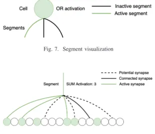
The visualization for the segments connection to cells is provided in Figure 7 and the illustration for the synapses connecting to segments is in Figure 8.

Fig. 7. Segment visualization

Fig. 8. Synapse visualization

Cells are connected to segments. The segments contain synapses that connect to other cells. A segment’s activation is also binary, either active or not. A segment becomes active if enough of its synapses become active, this can be solved as a summation across the segments.

In the Spatial Pooler, one cell has one segment connected to it, so this is just like in a normal neural network. In the Temporal Memory, one cell has multiple segments connected to is. If any segment is activated, the cell becomes active as well. This is like an or operation between the segment activations. One segment can be viewed as a recognizer for a similar subset of SDR representations.

Training of the HTM network is different from other neural networks. In the network, all neurons, segments, and synapses have binary activations. Since this network is binary, the typical loss backpropagation method will not work in this case.

The training suited for such a network is Hebbian learning.

It is a rather simple unsupervised training method, where the

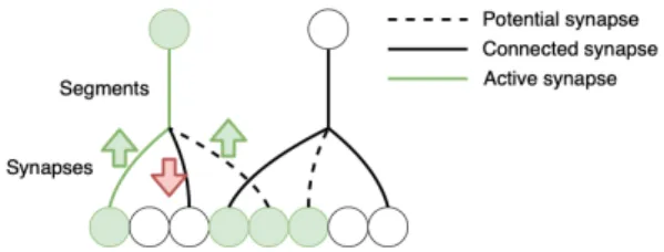
training occurs between neighboring layers only. The Hebbian learning is illustrated in Figure 9.

Fig. 9. Visualization of Hebbian learning

• Only those synapses that are connected to an active cell through a segment train.

• If one synapse is connected to an active cell, then it contributed right to the activation of that segment.

Therefore its strength should be incremented.

• If one synapse is connected to an inactive cell, then it did not contribute right to the activation of that segment.

Therefore its strength should be decreased.

C. HTM software solutions

There are HTM implementations maintained by Numenta, which give the foundation for other implementations.

First, the NuPIC Core (Numenta Platform for Intelligent Computing) is the C++ codebase of the official HTM projects.

It contains all HTM algorithms which can be used by other lan- guage bindings. Any further bindings should be implemented in this repository. This codebase implements the Network API, which is the primary interface for creating whole HTM systems. It will implement all algorithms for NuPIC but is currently under transition. The implementation is currently a failing build according to their CircleCI validation [19].

NuPIC is the Python implementation of the HTM algorithm.

It is also a Python binding to the NuPIC Core. This is the implementation we choose as baseline. In addition to the other repository’s Network API, this also has a High-level API called the Online Prediction Framework (OPF). Through this framework predictions can be made and also it can be also used for anomaly detection. To optimize the network’s hyper- parameters swarming can be implemented, which generates multiple network versions simultaneously. The C++ codebase can be used instead of the Python implementation if explicitly specified by the user [18].

There is also an official and community-driven Java version of the Numenta NuPIC implementation. This repository pro- vides a similar interface as the Network API from NuPIC and has comparable performance. The copyright was donated to the Numenta group by the author [20].

Comportex is also an official implementation of HTM using Clojure. It is not derived from NuPIC, it is a separate implementation, originally based on the CLA whitepaper [21], then also improved.

Comportex is more a library than a framework because of Clojure. The user controls simulations and can extract useful

network information like the set of active cells. These variables can be used to generate predictions or anomaly scores.²

There are also unofficial implementations, which are based on the CLA whitepaper or the Numenta HTM implementations.

• Bare Bone Hierarchical Temporal Memory (bbHTM)³

• pyHTM⁴

• HTM.core⁵

• HackTM⁶

• HTM CLA⁷

• CortiCL⁸

• Adaptive Sequence Memorizer⁹

• Continuous HTM¹⁰

• Etaler¹¹

• HTM.cuda¹²

• Sanity¹³

• Tiny-HTM¹⁴

III. PROPOSED METHOD

The goal of this work is to introduce sparse matrix operations to HTM networks to be able to realize larger models. Current implementations of the HTM network are not using sparse matrix operations, and these are using array-of-objects approach for storing cell connections. The proposed method is evaluated on two types of data: real consumption time-series and synthetic sinusoid data.

The first dataset is provided by Numenta called Hot Gym [22]. It consists of hourly power consumption values measured in kWh. The dataset is more than 4000 measurements long and also comes with timestamps. By plotting the data the daily and weekly cycles are clearly visible.

The second dataset is created by the timesynth Python package producing 5000 data points of a sinusoid signal with Gaussian noise.

A matrix implementation collects the segment and synapse connections in an interpretable data format compared to the array-of-objects approaches. The matrix implementation

2Comportex (Clojure), https://github.com/htm-community/comportex, Ac- cess date: 14th April 2020

3https://github.com/vsraptor/bbhtm, Access date: 14th April 2020

4pyHTM, https://github.com/carver, Access date: 14th April 2020

5htm.core, https://github.com/htm-community/htm.core, Access date: 14th April 2020

6HackTMM, https://github.com/glguida/hacktm, Access date: 14th April 20207HTM CLA, https://github.com/MichaelFerrier/HTMCLA, Access date: 14th April 2020

8ColriCl, https://github.com/Jontte/CortiCL, Access date: 14th April 2020

9Adaptive Sequence Memorizer, (ASM),https://github.com/ziabary/Adaptive- Sequence-Memorizer, Access date: 14th April 2020

10Continuous HTM GPU (CHTMGPU),

https://github.com/222464/ContinuousHTMGPU, Access date: 14th April 202011Etaler, https://github.com/etaler/Etaler, Access date: 14th April 2020

12HTM.cuda, https://github.com/htm-community/htm.cuda, Access date: 14th April 2020

13Sanity, https://github.com/htm-community/sanity, Access date: 14th April 202014Tiny-HTM, https://github.com/marty1885/tiny-htm, Access date: 14th April 2020

(5)

4Comportex (Clojure), https://github.com/htm-community/comportex, Access date: 14th April 2020

8HackTMM, https://github.com/glguida/hacktm, Access date: 14th April 2020

9HTM CLA, https://github.com/MichaelFerrier/HTMCLA, Access date:

14th April 2020

11Adaptive Sequence Memorizer, (ASM),https://github.com/ziabary/

Adaptive-Sequence-Memorizer, Access date: 14th April 2020

12Continuous HTM GPU (CHTMGPU), https://github.com/222464/

ContinuousHTMGPU, Access date: 14th April 2020

13Etaler, https://github.com/etaler/Etaler, Access date: 14th April 2020

14HTM.cuda, https://github.com/htm-community/htm.cuda, Access date:

14th April 2020

15Sanity, https://github.com/htm-community/sanity, Access date: 14th April 2020

16Tiny-HTM, https://github.com/marty1885/tiny-htm, Access date: 14th April 2020

4) Temporal Memory: The Temporal Memory receives the active columns as input and outputs the active cells which represent the context of the input in those active columns. At any given timestep the active columns tell what the network sees and the active cells tell in what context the network sees it.

A visualization of the Temporal Memory columns cells and connections is provided in Figure 6.

Fig. 6. Temporal Memory connections

The cells in the Temporal Memory are binary, active or inactive. Additionally, the network’s cells can be in a predictive state based on their connections, which means activation is anticipated in the next timestep for that cell. The cells inside every column are also competing for activation. A cell is activated if it is in an active column and was in a predictive state in the previous timestep. The other cells can’t get activated because of the inhibition.

The connections in the Temporal Memory between cells are created during training, not initialized like in the Spatial Pooler. When there is an unknown pattern none of the cells become predictive in a given column. In this case bursting happens. Bursting expresses the union of all possible context representation in a column, so expresses that the network does not know the context. To later recognize this pattern a winner cell is needed to choose to represent the new pattern the network encountered. The winner cells are chosen based on two factors, matching segments and least used cells.

• If there is a cell in the column that has a matching segment, it was almost activated. Therefore it should be the representation of this new context.

• If there is no cell in the column with a matching segment, the cell with the least segments should be the winner.

The training happens similarly to Spatial Pooler training.

The difference is that one cell has many segments connected to it, and the synapses of these segments do not connect to the previous layer’s output but other cells in the temporary memory. The training also creates new segments and synapses to ensure that the unknown patterns get recognized the next time the network encounters them.

The synapse reinforcement is made on the segment that led to the prediction of the cell. The synapses of that segment are updated. Also if there were not enough active synapses, the network grows new ones to previous active cells to ensure at least the desired amount of active synapses.

In the case where the cell is bursting the training is different.

One cell must be chosen as winner cell. This cell will grow a

new segment, which in turn will place the cell in a similar situation into the desired predictive state. The winner cell can be the most active cell, that almost got into predictive state, or the lowest utilized, in other words the cell that has the fewest segments. Only winner cells are involved in the training process. Correctly predicted cells are automatically winner cells as well, so those are always trained. The new segment will connect to some of the winner cells in the previous timestep.

5) Segments, synapses and training: In the HTM network segments and synapses connect the cells. Synapses start as potential synapses. This means that a synapse is made to a cell, but not yet strong enough to propagate the activation of the cell. During training, this strength can change and above the threshold the potential synapse becomes connected. A synapse is active if it is connected to an active cell.

The visualization for the segments connection to cells is provided in Figure 7 and the illustration for the synapses connecting to segments is in Figure 8.

Fig. 7. Segment visualization

Fig. 8. Synapse visualization

Cells are connected to segments. The segments contain synapses that connect to other cells. A segment’s activation is also binary, either active or not. A segment becomes active if enough of its synapses become active, this can be solved as a summation across the segments.

In the Spatial Pooler, one cell has one segment connected to it, so this is just like in a normal neural network. In the Temporal Memory, one cell has multiple segments connected to is. If any segment is activated, the cell becomes active as well. This is like an or operation between the segment activations. One segment can be viewed as a recognizer for a similar subset of SDR representations.

Training of the HTM network is different from other neural networks. In the network, all neurons, segments, and synapses have binary activations. Since this network is binary, the typical loss backpropagation method will not work in this case.

The training suited for such a network is Hebbian learning.

It is a rather simple unsupervised training method, where the

training occurs between neighboring layers only. The Hebbian learning is illustrated in Figure 9.

• pyHTM⁴

• HTM.core⁵

• HackTM⁶

• HTM CLA⁷

• CortiCL⁸

• Etaler¹¹

• HTM.cuda¹²

• Sanity¹³

• Tiny-HTM¹⁴

The goal of this work is to introduce sparse matrix operations to HTM networks to be able to realize larger models.

Current implementations of the HTM network are not using sparse matrix operations, and these are using array-of-objects approach for storing cell connections. The proposed method is evaluated on two types of data: real consumption time-series and synthetic sinusoid data.

6HackTMM, https://github.com/glguida/hacktm, Access date: 14th April 20207HTM CLA, https://github.com/MichaelFerrier/HTMCLA, Access date:

14th April 2020

network information like the set of active cells. These variables can be used to generate predictions or anomaly scores.⁴

There are also unofficial implementations, which are based on the CLA whitepaper or the Numenta HTM implementations.

 Bare Bone Hierarchical Temporal Memory (bbHTM)³  pyHTM⁴

 HTM.core⁵  HackTM⁶  HTM CLA⁷  CortiCL⁸

 Adaptive Sequence Memorizer⁹  Continuous HTM¹⁰

 Etaler¹¹  HTM.cuda¹²  Sanity¹³  Tiny-HTM¹⁴ training occurs between neighboring layers only. The Hebbian

learning is illustrated in Figure 9.

• pyHTM⁴

• HTM.core⁵

• HackTM⁶

• HTM CLA⁷

• CortiCL⁸

• Etaler¹¹

• HTM.cuda¹²

• Sanity¹³

• Tiny-HTM¹⁴

The goal of this work is to introduce sparse matrix operations to HTM networks to be able to realize larger models.

Current implementations of the HTM network are not using sparse matrix operations, and these are using array-of-objects approach for storing cell connections. The proposed method is evaluated on two types of data: real consumption time-series and synthetic sinusoid data.

6HackTMM, https://github.com/glguida/hacktm, Access date: 14th April 20207HTM CLA, https://github.com/MichaelFerrier/HTMCLA, Access date:

14th April 2020