Additive and multiplicative properties of scoring methods for preference aggregation by László Csató
C O R VI N U S E C O N O M IC S W O R K IN G P A PE R S
http://unipub.lib.uni-corvinus.hu/1562
CEWP 3 /2014
Additive and multiplicative properties of scoring methods for preference aggregation ∗
L´ aszl´ o Csat´ o
†Department of Operations Research and Actuarial Sciences Corvinus University of Budapest
MTA-BCE ”Lend¨ulet” Strategic Interactions Research Group Budapest, Hungary
May 15, 2014
Abstract
The paper reviews some additive and multiplicative properties of ranking pro- cedures used for generalized tournaments with missing values and multiple compar- isons. The methods analysed are the score, generalised row sum and least squares as well as fair bets and its variants. It is argued that generalised row sum should be applied not with a fixed parameter, but a variable one proportional to the number of known comparisons. It is shown that a natural additive property has strong links to independence of irrelevant matches, an axiom judged unfavourable when players have different opponents.
JEL classification number: D71
Keywords: Preference aggregation, Tournament ranking, Paired comparison, Ax- iomatic approach
1 Introduction
Paired-comparison based ranking problems are given by a set of objects and a tournament matrix, which represents the performance of objects against each other. They arise in many different fields like social choice theory (Chebotarev and Shamis, 1998), sports (Landau, 1895, 1914; Zermelo, 1928) or psychology (Thurstone, 1927). The usual goal is to determine a winner (a set of winners) or a complete ranking for the objects. There were some attempts to link the two areas (i.e. Bouyssou (2004)), however, their results seem to be limited. We will deal only with the latter problem, allowing for different preference intensities (including ties), incomplete and multiple comparisons among the objects.
Ranking procedures are usually given as functions associating a score for each object and a higher score corresponds to a better ranking. The literature on these methods has expanded significantly (for reviews, see Laslier (1997) and Chebotarev and Shamis
∗We are grateful to Julio Gonz´alez-D´ıaz for his remark about homogeneity.
†e-mail: laszlo.csato@uni-corvinus.hu
(1998)), so there is a real need for some guidelines about the choice of the appropriate procedure. It may be achieved by studying their axiomatic properties. Characterization results on this general domain are limited, we know them only for fair bets (Slutzki and Volij, 2005) and invariant methods (Slutzki and Volij, 2006). Our goal is to investigate some scoring procedures with respect to a set of properties, naturally arising from the setting. Our results supplement Gonz´alez-D´ıaz et al. (2014)’s findings by analysing new methods and axioms.
Because of the large amount of ranking methods discussed in the different fields, some selection is needed. We will mainly concentrate on the following procedures.
• Score: a natural method for binary tournaments (for characterizations on re- stricted domains, see Young (1974); Hansson and Sahlquist (1976); Rubinstein (1980); Nitzan and Rubinstein (1981); Bouyssou (1992)).
• Least squares: a well-known procedure in statistics and psychology (see Thur- stone (1927); Gulliksen (1956); Kaiser and Serlin (1978)).
• Generalised row sum: a parametric family of ranking methods resulting in the score and least squares as limits (see Chebotarev (1989, 1994)).
• Fair bets: an extensively studied method in social choice theory as well as for ranking the nodes of directed graphs (see Daniels (1969); Moon and Pullman (1970); Slutzki and Volij (2005, 2006); Slikker et al. (2012)).
• Dual fair bets: a scoring procedure obtained from fair bets by ’reversing’ an axiom in its characterization (see Slutzki and Volij (2005)).
• Copeland fair bets: a new method introduced in the current paper by ap- plying the idea of Herings et al. (2005) for fair bets.
The main contribution of this paper is to study the ranking methods above in the view of a set of axioms. It helps in understanding the different procedures and reveals the connections of the properties investigated. For instance, Copeland fair bets is proposed because Gonz´alez-D´ıaz et al. (2014) considers that its major weakness is the violation of inversion, which imposes the requirement that if all the results are reversed, then the corresponding ranking should be obtained by reversing the original ranking as well. The significance of certain axioms for applications will also be emphasized. Thorough analysis of these properties may support the work towards the characterization of some methods, too.
The paper is structured as follows. In Section 2 our setting and definitions are pre- sented. Section 3 exhibits three main properties with a significance for later discussion. In Section 4 we deal with two possible multiplicative axioms. Section 5 reviews four axioms linked to adding of ranking problems. In Section 6, we argue that the strongest additive property has unfavourable implications on the general domain used. Finally, Section 7 concludes the results, summarized visually in a table and a graph.
2 Notations and rating methods
Let N = {X1, X2, . . . , Xn}, n ∈ N be a set of objects and A = (aij) ∈ Rn×n be a tournament matrix such that aij +aji ∈ N. aij represents the aggregate score of object
Xi againstXj,aij/(aij+aji) may be interpreted as the likelihood that object Xi is better than object Xj. aii = 0 is assumed for all i = 1,2, . . . , n, diagonal entries will have no significance in the discussion. A possible derivation of the tournament matrix can be found in Gonz´alez-D´ıaz et al. (2014) and Csat´o (2014). This notation also follows Chebotarev and Shamis (1998).
The pair (N, A) is called a ranking problem.1 The set of ranking problems is denoted by R. A scoring procedure f is an R → Rn function, fi = fi(N, A) is the rating of object Xi. It immediately determines a ranking (transitive and complete weak order on the set N ×N) , where fi ≥fj means that Xi is ranked weakly above Xj, denoted by Xi Xj. Ratings provide cardinal and rankings provide ordinal information about the objects. Throughout the paper, the notions of rating and ranking methods will be used analogously since only scoring procedures are discussed.
To each ranking problem (N, A) ∈ R, we associate a results matrix R = A−A> = (rij)∈Rn×nand amatches matrix M =A+A> = (mij)∈Nn×n, wheremij is the number of the comparisons betweenXi andXj, whose the outcome is given byrij. di =Pn
j=1mij is the total number of comparisons of object Xi. m = maxXi,Xj∈Nmij is the maximal number of comparisons in the ranking problem. A ranking problem is called round-robin if mij =m for all Xi 6=Xj, namely, every object has been compared with all the others exactly as many times. The set of round-robin ranking problems is denoted by RR. Note that ranking problem can be also defined by matrices R and M with the restriction
|rij| ≤mij for all Xi, Xj ∈N.
Ranking of the objects involves three main challenges. The first one is the possible appearance of circular triads, when object Xi is better than Xj (that is,aij > aji), Xj is better than Xk, but Xk is better than Xi. If preference intensities also count as in the model above, other triplets (Xi, Xj, Xk) may produce problems, too. The second problem is that the performance of objects compared with Xi strongly influences the observable paired comparison outcomes aij. For example, if Xi was compared only with Xj, then its rating may depend on the results of Xj. The third difficulty is given by the different number of comparisons of the objects, di 6= dj. According to David (1987, p. 1), it must be realized that there can be no entirely satisfactory way of ranking if the number of replications of each object varies appreciably. Despite this we do not deal with the question whether a given dataset may be globally ranked in a meaningful way or the data is inherently inconsistent, an issue investigated for example by Jiang et al. (2011). Since each problem occur if n ≥3, the case of two objects becomes trivial.
MatrixM can be represented by an undirected multigraph G:= (V, E) where vertex setV corresponds to the object setN, and the number of edges between objectsXiandXj is equal to mij. Therefore the degree of node Xi is di. Graph G is called thecomparison multigraph associated with the ranking problem (N, R, M), however, it is independent of the results matrix R. The Laplacian matrix L = (`ij), i, j = 1,2, . . . , n of graph G is given by `ij =−mij for all Xi 6=Xj and `ii =di for all Xi ∈N.
Apath fromXk1 toXkt is a sequence of objectsXk1, Xk2, . . . , Xkt such thatmk`k`+1 >0 for all `= 1,2, . . . , t−1. Two objects are connected if there exists a path between them.
Ranking problem (N, A)∈ R is said to beconnected if every pair of objects is connected.
The set of connected ranking problems is denoted by RC.
A directed path from Xk1 to Xkt is a sequence of objects Xk1, Xk2, . . . , Xkt such that ak`k`+1 > 0 for all ` = 1,2, . . . , t−1. Objects Xi and Xj are in the same league if there
1 In certain cases we will denote it only by the tournament matrixA, whose rows already determine the set of objects N.
exists a directed path from Xi to Xj and from Xj to Xi. Ranking problem (N, A)∈ R is called irreducible if every pair of objects is in the same league. The set of irreducible ranking problems is denoted by RI.
Let e ∈ Rn be the unit column vector, that is, ei = 1 for all i = 1,2, . . . , n. Let I ∈ Rn×n be the identity matrix, and L be the Laplacian matrix of the comparison multigraph Gassociated with the ranking problem (N, A).
Now we define some rating methods. The first one does not take the comparison structure into account.
Definition 2.1. Score: s(N, R, M) =Re.
Score will also be referred to asrow sum. The following parametric rating method was constructed axiomatically by Chebotarev (1989) and thoroughly analyzed in Chebotarev (1994).
Definition 2.2. Generalized row sum: it is the unique solution x(ε)(N, R, M) of the system of linear equations (I +εL)x(ε)(N, R, M) = (1 +εmn)s, where ε > 0 is a parameter.
It adjusts the standard scoresi by accounting for the performance of objects compared withXi, and adds an infinite depth to this argument since scores of all objects available on a path appear in the calculation. εindicates the importance attributed to this correction.
An alternative solution would be to count only the scores of direct opponents as in David (1987).
Lemma 2.1. Generalised row sum results in row sum if ε→0: limε→0x(ε)(N, R, M) = s(N, R, M).
There are few information about the choice of parameterε. In our case, the value of rij is limited by −mij and mij, thus some conditions can be made on ε.
Definition 2.3. Reasonable choice of ε (Chebotarev, 1994, Proposition 5.1): Let (N, R, M) ∈ R be a ranking problem. Reasonableness for the choice of ε amounts to satisfying the constraint
0< ε≤ 1 m(n−2). Reasonable upper bound of ε is 1/[m(n−2)].
The reasonable choice is not well-defined in the trivial case of n = 2, thus n ≥ 3 is implicitly assumed in the following.
Proposition 2.1. For the generalised row sum method with a reasonable choice of ε,
−m(n−1)≤xi(ε)(N, R, M)≤m(n−1) for all Xi ∈N. Proof. See Chebotarev (1994, Property 13).
It is favourable as in a round-robin ranking problem −m(n −1) ≤ si(N, R, M) ≤ m(n−1) for all Xi ∈N.
Both the score and generalized row sum ratings are well-defined and easily computable from a system of linear equations for all ranking problems (N, R, M)∈ R.
The least squares method was suggested by Thurstone (1927) and Horst (1932). Other references can be found in Csat´o (2014).
Definition 2.4. Least squares: it is the solution q(N, R, M) of the system of linear equations Lq(N, R, M) =s(N, R, M) and e>q(N, R, M) = 0.
Lemma 2.2. Generalised row sum results in least squares if ε→ ∞:
ε→∞lim x(ε)(N, R, M) =mnq(N, R, M).
Proposition 2.2. The least squares rating is unique if and only if comparison multigraph G is connected.
Proof. See Boz´oki et al. (2014). Chebotarev and Shamis (1999, p. 220) mention this fact without further discussion.
An extensive analysis and a graph interpretation of the least squares method can be found in Csat´o (2014).
Several scoring procedures build upon the idea of rewarding wins without punishing losses. Two early contributions in this field are Wei (1952) and Kendall (1955). They have been studied in social choice and game theory by Borm et al. (2002); Herings et al. (2005);
Slikker et al. (2012); Slutzki and Volij (2005, 2006). One of the most widely used method within this framework is the fair bets method, originally suggested by Daniels (1969) and Moon and Pullman (1970), and axiomatically characterized by Slutzki and Volij (2005) and Slutzki and Volij (2006). Its properties have been investigated by Gonz´alez-D´ıaz et al.
(2014).
Let F = diag(A>e), an n ×n diagonal matrix with the number of losses for each object.
Definition 2.5. Fair bets: it is the solution fb(N, A) of the system of linear equations F−1Afb(N, A) = fb(N, A) and e>fb(N, A) = 1.
Proposition 2.3. The fair bets rating is unique if the ranking problem is irreducible.
Proof. See Moon and Pullman (1970).
For reducible ranking problems, Perron-Frobenius theorem does not guarantee that the eigenvector corresponding to the dominant eigenvalue is strictly positive.
Therefore we restrict our analysis to the class of connected ranking problemsRC, and to the set of irreducible ranking problemsRI in the case of fair bets. However, for ranking problems without a connected comparison multigraph, rating of all objects on a common scale seems to be arbitrary.
The idea behind the fair bets method is to give more weight to wins against better objects than to losses against worse objects. It includes a subjective judgement in it:
analogously, one may argue that the latter is more favourable. This approach is taken by the dual fair bets method (Slutzki and Volij, 2005) using the transposed tournament matrix A>, however, in this case a lower value is better.
Definition 2.6. Dual fair bets: it is the opposite of the solution dfb∗(N, A) of system of linear equations [diag(Ae)]−1A>dfb∗(N, A) =dfb∗(N, A) and e>dfb∗(N, A) = 1.
The transformation dfb(N, A) = −dfb∗(N, A) is necessary in order to ensure that Xi Xj ⇔df bi(N, A)≥df bj(N, A) for all Xi, Xj ∈N.
In fact, the axiomatization of fair bets also characterizes the dual fair bets by chang- ing only one property, negative responsiveness to losses with positive responsiveness to
wins (Slutzki and Volij, 2005, Remark 1). This differentiation can be seen in the case of positional power, too, by the definition of positional power and positional weakness (Her- ings et al., 2005). Similarly to the latter paper’s Copeland positional value, we introduce Copeland fair bets method.
Definition 2.7. Copeland fair bets: Cfb(N, A) it is the sum of the fair bets and dual fair bets ratings, Cfb(N, A) = Cfb(N, A) +dfb(N, A).
Now Xi Xj ⇔ Cf bi(N, A) ≥ Cf bj(N, A) as earlier. According to our knowledge, we are the first to define this scoring procedure.
These are the six scoring procedures (or, in the case of generalised row sum, a family of them) discussed in the article. Gonz´alez-D´ıaz et al. (2014) have analysed the least squares and fair bets methods, as well as generalised row sum with the parameter ε = 1/[m(n−2)]. They use a different version of the score, si/di for all Xi ∈N.
Ranking problem (N, R, M)∈ R can be represented by a graph such that the nodes are the objects, k times (Xi, Xj)∈N×N undirected edge means rij(= rji) = 0,mij =k, and k times (Xi, Xj) ∈ N ×N directed edge means rij = k (rji = −k), mij = k. We think it helps a lot in understanding the examples.
Figure 1: Ranking problem of Example 1
X1 X2
X3
X4 X5
Example 1. (Chebotarev, 1994, Example 2) Let (N, R, M) ∈ R be the ranking problem in Figure 1 with the set of objects N ={X1, X2, X3, X4, X5}.
The corresponding tournament, results and matches matrices are as follows
A =
0 0 0 0 1
0 0 0.5 0 0 0 0.5 0 1 0
0 0 0 0 1
0 0 1 0 0
, R =
0 0 0 0 1
0 0 0 0 0
0 0 0 1 −1
0 0 −1 0 1
−1 0 1 −1 0
, M =
0 0 0 0 1 0 0 1 0 0 0 1 0 1 1 0 0 1 0 1 1 0 1 1 0
.
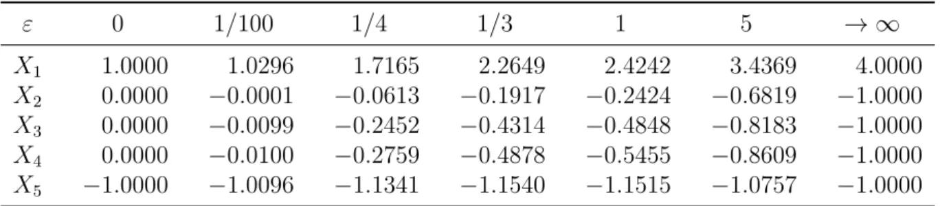
The solutions with generalised row sum for various values ofε are given in Table 1.
Herem= 1 andn = 5, thus ε= 1/3 is the reasonable upper bound. For all parameter greater than 0, the ranking is X1 X2 X3 X4 X5 since X1 dominates X5, which effectsX3 andX4 through the circular triad(X3, X4, X5). However,X3 has a draw against X2. Note that X2 ∼X3 ∼X4 for the score and least squares methods, referring to a kind of neglect of the comparison (X2, X3).
It is an irreducible ranking problem, so fair bets rating is not unique. Nevertheless, a ranking can be obtained by the application of its extension according to Slutzki and Volij (2005): X1 is the best object as no other has a chance to defeat it, and the remaining four
Table 1: x(ε) rating vectors of Example 1
ε 0 1/100 1/4 1/3 1 5 → ∞
X1 1.0000 1.0296 1.7165 2.2649 2.4242 3.4369 4.0000
X2 0.0000 −0.0001 −0.0613 −0.1917 −0.2424 −0.6819 −1.0000 X3 0.0000 −0.0099 −0.2452 −0.4314 −0.4848 −0.8183 −1.0000 X4 0.0000 −0.0100 −0.2759 −0.4878 −0.5455 −0.8609 −1.0000 X5 −1.0000 −1.0096 −1.1341 −1.1540 −1.1515 −1.0757 −1.0000
form an irreducible component. It gives the fair bets ranking as X1 (X2 ∼X3 ∼ X4 ∼ X5), which coincides with the one from least squares. Similarly, both dual fair bets and Copeland fair bets result in X1 (X2 ∼X3 ∼X4 ∼X5).
3 Structural invariance properties
Our axiomatic discussion begins with some basic properties already known from the lit- erature.
Definition 3.1. Neutrality (N EU) (Young, 1974): Let (N, R, M) ∈ R be a ranking problem andσ :N →N be a permutation on the set of objects. Letσ(N, R, M)∈ R be the ranking problem obtained from(N, R, M) by this permutation. Scoring proceduref :R → Rn is neutral if for all Xi, Xj ∈ N: fi(N, R, M) ≥ fj(N, R, M) ⇔ fσi[σ(N, R, M)] ≥ fσj[σ(N, R, M)].
In some articles, it is called anonymity (Bouyssou, 1992; Slutzki and Volij, 2005;
Gonz´alez-D´ıaz et al., 2014). It is equivalent with requiring that the permutation of two objects do not affect the ranking as in Gonz´alez-D´ıaz et al. (2014).
Remark 1. Let f :R →Rn be a neutral scoring procedure. If for the objectsXi, Xj ∈N, mij = 0, and rik = rjk, mik = mjk for all Xk ∈ N \ {Xi, Xj}, then fi(N, R, M) = fj(N, R, M) (Bouyssou, 1992, p. 62).
Lemma 3.1. All methods presented above satisfy N EU.
Definition 3.2. Symmetry (SY M) (Gonz´alez-D´ıaz et al., 2014): Let (N, R, M) ∈ R be a ranking problem such that R = 0. Scoring procedure f : R → Rn is symmetric if fi(N, R, M) =fj(N, R, M) for all Xi, Xj ∈N.
Symmetry does not requiredi =dj for the pair (Xi, Xj). Young (1974) and Nitzan and Rubinstein (1981, Axiom 4) use the axiomcancellation for round-robin ranking problems, which coincides with symmetry on this set.
Lemma 3.2. All methods presented above satisfy SY M.
Definition 3.3. Inversion (IN V) (Chebotarev and Shamis, 1998): Let (N, R, M) ∈ R be a ranking problem. Scoring procedure f : R → Rn is invertible if fi(N, R, M) ≥ fj(N, R, M)⇔fi(N,−R, M)≤fj(N,−R, M) for all Xi, Xj ∈N.
Inversion means that taking the opposite of each result changes the ranking accord- ingly. It establishes a uniform treatment of victories and defeats. Chebotarev (1994, Property 7) defines transposability such that the ratings change their sign and keep the same absolute value.
Remark 2. Let f :R →Rn be a scoring procedure satisfying IN V. Then fi(N, R, M)>
fj(N, R, M)⇔fi(N,−R, M)< fj(N,−R, M) for all Xi, Xj ∈N.
The following result is mentioned by Gonz´alez-D´ıaz et al. (2014, p. 150).
Corollary 1. IN V implies SY M.
Lemma 3.3. The score, generalised row sum and least squares methods satisfy IN V. Proof. It is the immediate consequence of s(N,−R, M) =−s(N, R, M).
Lemma 3.4. Fair bets and dual fair bets methods do not satisfy IN V on the set RR. Proof. For fair bets, see Gonz´alez-D´ıaz et al. (2014, Example 4.4). The same counterex- ample with a transposed tournament matrix proves the statement for dual fair bets.
So axiom IN V is not satisfied by the two methods still on the restricted domain of round-robin problems.
Lemma 3.5. Copeland fair bets satisfies IN V.
Proof. Take ranking problems (N, A) and (N, A>). Cfb(N, A) =fb(N, A) +dfb(N, A) =
−dfb(N, A>)−fb(N, A>) =−Cfb(N, A>).
Hence Copeland fair bets eliminates the major weakness of fair bets according to Gonz´alez-D´ıaz et al. (2014, p. 164), while retains its favourable properties.
4 Multiplicative properties
The following axiom refers to proportional modification of the ranking problem.
Definition 4.1. Homogeneity (HOM) (Gonz´alez-D´ıaz et al., 2014): Let (N, R, M)∈ R be a ranking problem and k >0 such that (N, kR, kM)∈ R. Scoring procedure f :R → Rn is homogeneous, if fi(N, R, M) ≥ fj(N, R, M) ⇔ fi(N, kR, kM) ≥ fj(N, kR, kM) for all Xi, Xj ∈N.2
In our setting the elements of kM should be integers, which is not required by Gonz´alez-D´ıaz et al. (2014).
Lemma 4.1. The score and least squares methods satisfy HOM.
Generalised row sum should be examined with some caution since it is a whole family of scoring procedures. First, we regard it with a constant parameter ε.
Proposition 4.1. The generalised row sum method with a fixed ε violates HOM.
Proof.
2 Since k >0, positive homogeneity may be a better name for this axiom, but we wanted to retain the original definition.
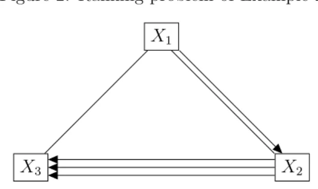
Figure 2: Ranking problem of Example 2 X1
X2 X3
Example 2. Let(N, R, M)∈ Rbe the ranking problem in Figure 2 with the set of objects N ={X1, X2, X3} and tournament matrix
A=
0 1.5 1 0.5 0 3 0.5 0 0
.
Let k= 2.
Here m = 3 and n = 3, the reasonable upper bound of ε is 1/3. Let choose it as a fixed parameter:
x(1/5)(N, R, M) = [2.0000; 2.0000; −4.0000]>, and x(1/5)(N,2R,2M) = [4.5352; 3.9437; −8.4789]>, implying X1 ∼x(1/3)(N,R,M) X2 but X1 x(1/3)(N,2R,2M)X2.
Now allow ε to depend on the matches matrix M.
Proposition 4.2. The generalised row sum method with a variable ε satisfies HOM if ε(k) is inversely proportional to k, that is, ε(k) = ε(1)/k =ε/k.
Proof. It yields from some basic calculations:
x(ε(k)) (N, kR, kM) = (1 +εmn)(I+εL)−1s(N, kR, kM) =kx(ε)(N, R, M).
Remark 3. The reasonable upper bound ε= 1 [m(n−2)] is inversely proportional to k.
Conjecture 1. The proof of Proposition 4.2 suggests that generalised row sum violates HOM if ε is not inversely proportional to k.
Lemma 4.2. Fair bets, dual fair bets and Copeland fair bets methods satisfy HOM. Proof. Regarding fair bets, fb(N, kA) = fb(N, A) since (kF)−1 = (1/k)F−1. It shows the homogeneity of dual fair bets as well, which proves HOM for Copeland fair bets.
It makes sense to deal only with the multiplication of results.
Definition 4.2. Admissible transformation of the results: Let (N, R, M)∈ R be a rank- ing problem. An admissible transformation of the results provides a ranking problem (N, kR, M)∈ R such that k >0, k∈R and krij ∈[−mij, mij] for all Xi, Xj ∈N.
k cannot be arbitrarily large in order to retain the condition|rij| ≤mij. For instance, in Example 2 maxXi,Xj∈Nrij/mij = max{1/3; 3/5} = 3/5, therefore 0 < k ≤ 5/3 makes (N, kR, M)∈ Ra ranking problem provided through an admissible transformation of the results. On the other hand, 0< k≤1 is always possible.
Definition 4.3. Scale invariance (SI): Let (N, R, M),(N, kR, M) ∈ R be two rank- ing problems such that (N, kR, M) is obtained from (N, R, M) through an admissible transformation of the results. Scoring procedure f : R → Rn is scale invariant if fi(N, R, M)≥fj(N, R, M)⇔fi(N, kR, M)≥fj(N, kR, M) for all Xi, Xj ∈N.
Scale invariance implies that the ranking is invariant to a proportional modification of wins (rij > 0) and losses (rij < 0). It seems to be important for applications. If the paired comparison outcomes cannot be measured on a continuous scale, it is not trivial how to transform them into rij values. SI provides that it is not a problem in several cases. For example, if only three outcomes are possible, the coding (rij = κ for wins;
rij = 0 for draws; rij = −κ for losses) makes the ranking independent from κ. It may be advantageous, too, when relative intensities, such as a regular win is two times better than an overtime triumph, are known.
Remark 4. Take the tournament matrix A, where aij = (rij + mij)/2. Through an admissible transformation of the results, every reducible A can be made irreducible (by all k < 1) if the ranking problem is connected.
Remark 4 offers a way to extend scale invariant scoring procedures unique on the domain RI toRC.
Lemma 4.3. The score, generalised row sum and least squares methods satisfy SI.
Proof. It is the immediate consequence of s(N, kR, M) =ks(N, R, M).
Proposition 4.3. Fair bets, dual fair bets and Copeland fair bets methods violate SI.
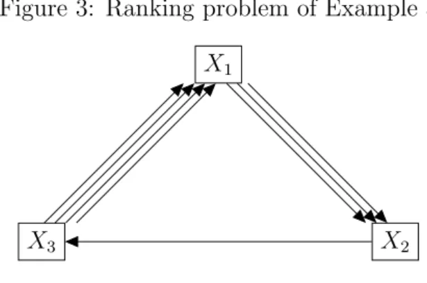
Figure 3: Ranking problem of Example 3 X1
X2 X3
Proof.
Example 3. Let (N, A) ∈ R be the ranking problem in Figure 3 with the set of objects N ={X1, X2, X3} and tournament matrix
A=
0 3 0 0 0 1 4 0 0
.
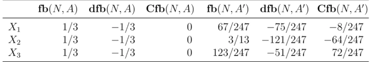
Table 2: Fair bets and associated rating vectors of Example 3
fb(N, A) dfb(N, A) Cfb(N, A) fb(N, A0) dfb(N, A0) Cfb(N, A0)
X1 1/3 −1/3 0 67/247 −75/247 −8/247
X2 1/3 −1/3 0 3/13 −121/247 −64/247
X3 1/3 −1/3 0 123/247 −51/247 72/247
Let k= 0.5, resulting in the tournament matrix A0 =
0 2.25 1 0.75 0 0.75
3 0.25 0
.
The rating vectors are given in Table 2. Thus f b1(N, A) ≤ f b2(N, A), df b1(N, A) ≤ df b2(N, A) and Cf b1(N, A) ≤ Cf b2(N, A), but f b1(N, A0) > f b2(N, A0), df b1(N, A0) >
df b2(N, A0) andCf b1(N, A0)> Cf b2(N, A0), which is a contradiction.
Similarly to Lemma 3.3, it is worth to examine the two multiplicative properties on the domain of round-robin ranking problems. Note that the set RR is closed under modifications allowed by HOM and SI (admissible transformation of the results).
Lemma 4.4. The generalised row sum satisfies HOM on the set RR.
Proof. Due to the axiomagreement (Chebotarev, 1994, Property 3), generalised row sum coincides with the score on this set of problems, so Lemma 4.1 holds.
Example 3 is unbalanced, the degree of the three nodes varies from 4 to 7. As it was mentioned in Section 2, in this case the ranking may be not meaningful. It also justifies the investigation of round-robin problems.
Proposition 4.4. Fair bets, dual fair bets and Copeland fair bets methods violate SI on the set RR.
Figure 4: Ranking problem of Example 4 X1
X2
X3 X4
Proof.
Example 4. Let (N, A) ∈ RR be the round-robin ranking problem in Figure 4 with the set of objects N ={X1, X2, X3, X4} and tournament matrix
A =
0 2 0 3 1 0 0 0 3 3 0 2 0 3 1 0
.
Let k= 0.5, resulting in the tournament matrix
A0 =
0 1.75 0.75 2.25 1.25 0 0.75 0.75 2.25 2.25 0 1.75 1.75 2.25 1.25 0
.
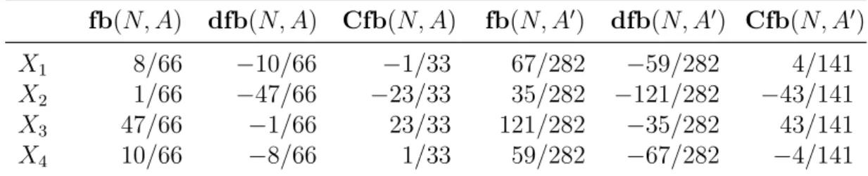
Table 3: Fair bets and associated rating vectors of Example 4
fb(N, A) dfb(N, A) Cfb(N, A) fb(N, A0) dfb(N, A0) Cfb(N, A0) X1 8/66 −10/66 −1/33 67/282 −59/282 4/141 X2 1/66 −47/66 −23/33 35/282 −121/282 −43/141
X3 47/66 −1/66 23/33 121/282 −35/282 43/141
X4 10/66 −8/66 1/33 59/282 −67/282 −4/141
The rating vectors are given in Table 3. Hence f b1(N, A)< f b4(N, A),df b1(N, A)<
df b4(N, A) and Cf b1(N, A) < Cf b4(N, A), but f b1(N, A0) > f b4(N, A0), df b1(N, A0) >
df b4(N, A0) andCf b1(N, A0)> Cf b4(N, A0), which proves the statement for fair bets and Copeland fair bets.
The other partial version of positive homogeneity, when matrix M is multiplied by k > 0, has no relevance. Moreover,HOM and SI already imply the respective property.
5 Additive properties
Definition 5.1. Consistency (CS) (Young, 1974): Let (N, R, M),(N, R0, M0) ∈ R be two ranking problems and Xi, Xj ∈ N be two objects. Let f : R → Rn be a scoring procedure such that fi(N, R, M) ≥ fj(N, R, M) and fi(N, R0, M0) ≥ fj(N, R0, M0). f is called consistent iffi(N, R+R0, M+M0)≥fj(N, R+R0, M+M0), moreover, fi(N, R+ R0, M +M0) > fj(N, R+R0, M +M0) if fi(N, R, M) > fj(N, R, M) or fi(N, R0, M0) >
fj(N, R0, M0).
CS is the most intuitive version of additivity.
Lemma 5.1. The score method satisfies CS.
Proposition 5.1. The generalised row sum and least squares methods violate CS.
Proof.
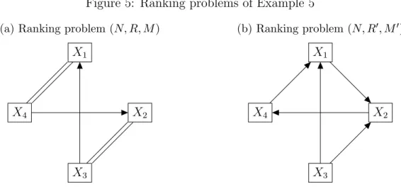
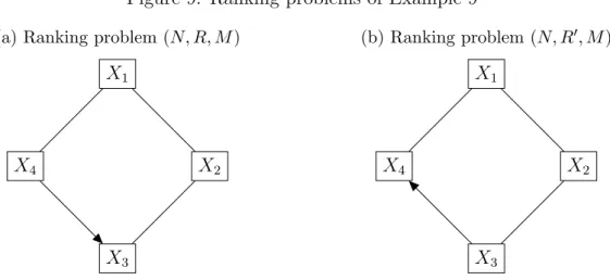
Figure 5: Ranking problems of Example 5 (a) Ranking problem (N, R, M)
X1
X2
X3 X4
(b) Ranking problem (N, R0, M0) X1
X2
X3 X4
Example 5. Let (N, R, M)∈ R and (N, R0, M0) ∈ R be the ranking problems in Figure 5 with the set of objects N ={X1, X2, X3, X4} and tournament matrices
A=
0 0 0 1 0 0 1 0 1 1 0 0 1 1 0 0
and A0 =
0 1 0 0 0 0 0 1 1 1 0 0 1 0 0 0
.
Let (N, R00, M00) = (N, R+R0, M+M0)∈ R be the sum of these two ranking problems.
Let x(ε)(N, R, M) = x(ε), x(ε)(N, R0, M0) = x(ε)0, x(ε)(N, R00, M00) = x(ε)00 and q(N, R, M) = q, q(N, R0, M0) = q0, q(N, R00, M00) = q00. Now n = 4, m =m0 = 1, thus m00= 2 and
x1(ε) = x2(ε) =−1 + 10ε+ 32ε2 + 32ε3 1 + 12ε+ 44ε2 + 48ε3, and x1(ε)0 =x2(ε)0 =−1, but
x1(ε)00−x2(ε)00=− 2ε+ 36ε2+ 160ε3
1 + 22ε+ 154ε2+ 340ε3 <0.
It implies that X1 ∼x(ε)(N,R,M)X2 and X1 ∼x(ε)(N,R0,M) X2, however, X1 ≺x(ε)(N,R00,M00) X2. Gener- alised row sum is not consistent for any ε.
Regarding the least squares method, on the basis of Lemma 2.2:
q1 = limε→∞x1(ε)
mn = limε→∞x2(ε)
mn =q2, and q10 = limε→∞x1(ε)0
m0n = limε→∞x2(ε)0
m0n =q20, but q100−q200 = limε→∞[x1(ε)00−x2(ε)00]
m00n =− 1 17 <0.
Hence X1 ∼q(N,R,M) X2 and X1 ∼q(N,R0,M0)X2 but X1 ≺q(N,R00,M00) X2.
Gonz´alez-D´ıaz et al. (2014, Example 4.2) have shown the violation of a somewhat weaker property called order preservation for the least squares and generalised row sum with ε= 1/[m(n−2)], since there di/dj =d0i/d0j for all Xi, Xj ∈N.
We will return later to the examination of fair bets and connected methods.
Gonz´alez-D´ıaz et al. (2014) discusses the following restricted version of additivity.
Definition 5.2. Flatness preservation (F P) (Slutzki and Volij, 2005): Let (N, R, M), (N, R0, M0) ∈ R be two ranking problems. Let f : R → Rn be a scoring procedure such that fi(N, R, M) =fj(N, R, M) and fi(N, R0, M0) = fj(N, R0, M0) for all Xi, Xj ∈ N. f preserves flatness if fi(N, R+R0, M+M0) = fj(N, R+R0, M +M0) for all Xi, Xj ∈N. Flatness preservation demands additivity only for problems with all objects ranked equally.
Corollary 2. CS implies F P.
Lemma 5.2. The score, generalised row sum and least squares methods satisfy F P. Proof. It has been shown in Gonz´alez-D´ıaz et al. (2014, Corollary 4.3) for the least squares, and in Gonz´alez-D´ıaz et al. (2014, Proposition 4.2) for generalised row sum with ε = 1/[m(n−2)].
The score method preserves flatness due to Lemma 5.1 and Corollary 2.
If xi(ε)(N, R, M) = xj(ε)(N, R, M) for all Xi, Xj ∈ N, then x(ε)(N, R, M) = 0. We prove that s(N, R, M) = 0 ⇔ x(ε)(N, R, M) = 0. si(N, R, M) = sj(N, R, M) for all Xi, Xj ∈ N impliess(N, R, M) =0, therefore x(ε)(N, R, M) =0. If x(ε)(N, R, M) = 0, then (1 +εmn)s=0, so s=0.
The same argument can be applied in the case of least squares.
Lemma 5.3. Fair bets, dual fair bets and Copeland fair bets methods satisfy F P.
Proof. Regarding the fair bets see Slutzki and Volij (2005, Theorem 1). According to Slutzki and Volij (2005, Remark 1), it is true for dual fair bets. It implies that Copeland fair bets preserves flatness.
All objects ranked equally seems to be a strong condition, so it makes sense to require additivity on a larger set. A natural choice can be that only the objects examined are ranked equally.
Definition 5.3. Equality preservation (EP): Let (N, R, M),(N, R0, M0) ∈ R be two ranking problems and Xi, Xj ∈N be two objects. Let f :R → Rn be a scoring procedure such that fi(N, R, M) = fj(N, R, M) and fi(N, R0, M0) = fj(N, R0, M0). f preserves equality if fi(N, R+R0, M +M0) = fj(N, R+R0, M +M0).
Corollary 3. CS implies EP. EP implies F P.
Lemma 5.4. The score method satisfies EP. Proof. It comes from Lemma 5.1 and Corollary 3.
Lemma 5.5. The generalised row sum and least squares methods violateEP.
Proof. x1(ε) = x2(ε) andq1 =q2as well asx1(ε)0 =x2(ε)0andq10 =q20, butx1(ε)00=x2(ε)00 and q100=q200 in Example 5.
Proposition 5.2. Fair bets, dual fair bets and Copeland fair bets methods violate EP. Proof.
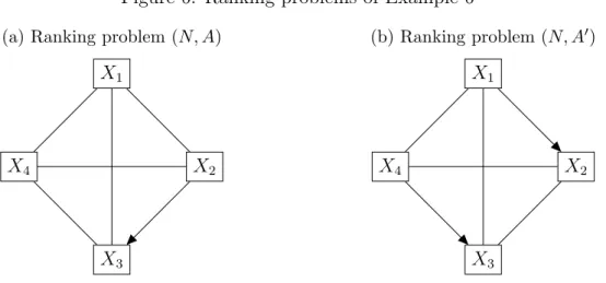
Figure 6: Ranking problems of Example 6 (a) Ranking problem (N, A)
X1
X2
X3 X4
(b) Ranking problem (N, A0) X1
X2
X3 X4
Example 6. Let (N, A) ∈ R and (N, A0) ∈ R be the ranking problems in Figure 6 with the set of objects N ={X1, X2, X3, X4} and tournament matrices
A =
0 0.5 0.5 0.5
0.5 0 1 0.5
0.5 0 0 0.5
0.5 0.5 0.5 0
and A0 =
0 1 0.5 0.5 0 0 0.5 0.5 0.5 0.5 0 0 0.5 0.5 1 0
.
Let (N, A00) = (N, A+A0)∈ R be the sum of these two ranking problems.
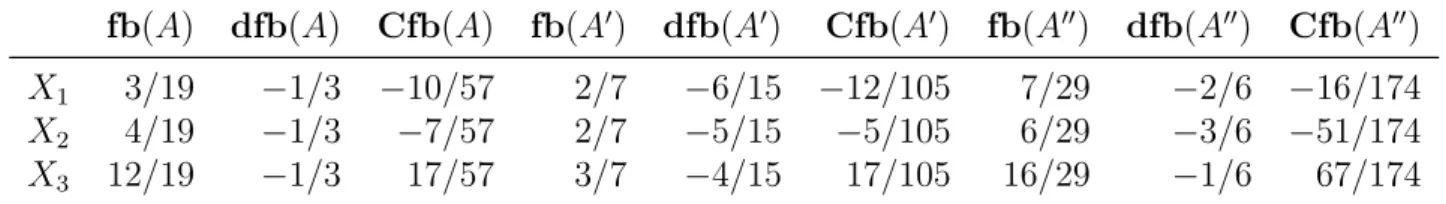
Table 4: Fair bets and associated rating vectors of Example 6
fb(A) dfb(A) Cfb(A) fb(A0) dfb(A0) Cfb(A0) fb(A00) dfb(A00) Cfb(A00)
X1 1/4 −1/4 0 3/8 −1/8 1/4 163/512 −101/512 31/256
X2 3/8 −1/8 1/4 1/8 −3/8 −1/4 117/512 −115/512 1/256
X3 1/8 −3/8 −1/4 1/8 −3/8 −1/4 75/512 −205/512 −65/256
X4 1/4 −1/4 0 3/8 −1/8 1/4 157/512 −91/512 33/256
The rating vectors are given in Table 4, where f b1(N, A) = f b4(N, A), df b1(N, A) = df b4(N, A), Cf b1(N, A) = Cf b4(N, A), similarly, f b1(N, A0) = f b4(N, A0), df b1(N, A0) = df b4(N, A0), Cf b1(N, A0) = Cf b4(N, A0), but f b1(N, A00) > f b4(N, A00), df b1(N, A00) <
df b4(N, A00), Cf b1(N, A00)< Cf b4(N, A00), which is a contradiction.
Lemma 5.6. Fair bets, dual fair bets and Copeland fair bets methods violate CS.
Proof. It comes from Proposition 5.2 with Corollary 3.
In the weakening of axiom CS, another natural restriction can be to allow only for the combination of ranking problems with the same matches matrix, when the effects of different comparison multigraphs are eliminated.
Definition 5.4. Result consistency (RCS): Let (N, R, M),(N, R0, M)∈ R be two rank- ing problems and Xi, Xj ∈ N be two objects. Let f : R → Rn be a scoring procedure such that fi(N, R, M)≥fj(N, R, M) and fi(N, R0, M)≥fj(N, R0, M). f is called result consistent if fi(N, R +R0,2M) ≥ fj(N, R +R0,2M), moreover, fi(N, R +R0,2M) >
fj(N, R+R0,2M) if fi(N, R, M)> fj(N, R, M) or fi(N, R0, M)> fj(N, R0, M).
Corollary 4. CS implies RCS.
Corollary 5. RCS (hence CS) implies HOM for all positive integer k.
Because of Corollary 5, generalised row sum with a constant value ofε= 1/3 violates of consistency according to Example 2 as k = 2.
Proposition 5.3. RCS and SY M implies IN V.
Proof. Take a ranking problem (N, R, M) ∈ R, assume that fi(N, R, M) ≥ fj(N, R, M) for objectsXi, Xj ∈N. Iffi(N,−R, M)> fj(N,−R, M), thenfi(N,0, M)> fj(N,0, M) due to RCS, which contradicts to SY M. Therefore fi(N,−R, M)≤fj(N,−R, M).
Corollary 6. CS and SY M implies IN V.
Corollary 6 was proved by Nitzan and Rubinstein (1981, Lemma 1) in the case of round-robin ranking problems.
Lemma 5.7. The score method satisfies RCS.
Proof. It comes from Lemma 5.1 and Corollary 4.
Proposition 5.4. The least squares method satisfies RCS.
Proof. Letq(N, R, M) = q,q(N, R0, M) =q0 andq(N, R+R0, M+M) = q00. It is shown that 2q00 =q+q0. The Laplacian matrix of the comparison multigraph associated with matches matrix M +M is 2L, so
2Lq00 =L(q+q0) = s(N, R, M) +s(N, R0, M) = s(N, R+R0, M +M) as well as e>q00=e>[(1/2)q+ (1/2)q0] = 0.
Regarding the generalised row sum, we repeatedly distinguish two cases.
Lemma 5.8. The generalised row sum method with a fixed ε violates RCS.
Proof. Corollary 5 can be applied because of k = 2 in Example 2.
Proposition 5.5. The generalised row sum method with a variable ε satisfies RCS if ε is inversely proportional to the number of added ranking problems.
Proof. Letx(ε)(N, R, M) =x(ε),x(ε)(N, R0, M) =x(ε)0 andx(ε)(N, R+R0, M+M) = x(ε)00. It yields from some basic calculations:
x(ε/2)00 = (1 +εmn)(I +εL)−1s(N, R+R0, M+M) =
= (1 +εmn)(I +εL)−1[s(N, R, M) +s(N, R0, M)] = x+x(ε)0.
Remark 5. The reasonable upper bound of ε = 1 [m(n−2)] is inversely proportional to the number of added ranking problems.
Conjecture 2. The proof of Proposition 5.5 suggests that generalised row sum violates HOM if ε is not inversely proportional to the number of added ranking problems.
Lemma 5.9. Fair bets and dual fair bets methods violate RCS.
Figure 7: Ranking problems of Example 7 (a) Ranking problem (N, A)
X1
X2 X3
(b) Ranking problem (N, A0) X1
X2 X3
Proof. It is a consequence of Lemmata 3.2 and 3.4 with Proposition 5.3.
Proposition 5.6. Copeland fair bets method violates RCS.
Proof.
Example 7. Let (N, A) ∈ R and (N, A0) ∈ R be the ranking problems in Figure 7 with the set of objects N ={X1, X2, X3} and tournament matrices
A=
0 3 0 0 0 1 4 0 0
and A0 =
0 1 2 2 0 0 2 1 0
with the same matches matrix
M =
0 3 4 3 0 1 4 1 0
.
Note that ranking problem(N, A)is the same as in Example 3. Let(N, A00) = (N, A+A0)∈ R be the sum of these two ranking problems.
Table 5: Fair bets and associated rating vectors of Example 7
fb(A) dfb(A) Cfb(A) fb(A0) dfb(A0) Cfb(A0) fb(A00) dfb(A00) Cfb(A00) X1 3/19 −1/3 −10/57 2/7 −6/15 −12/105 7/29 −2/6 −16/174 X2 4/19 −1/3 −7/57 2/7 −5/15 −5/105 6/29 −3/6 −51/174
X3 12/19 −1/3 17/57 3/7 −4/15 17/105 16/29 −1/6 67/174
The rating vectors are given in Table 5: Cf b1(N, A)< Cf b2(N, A) andCf b1(N, A0)<
Cf b2(N, A0), but Cf b1(N, A00)> Cf b2(N, A00).
Now we analyse the special case of round-robin ranking problems. Note that the set RR is closed under summation.
Lemma 5.10. The generalised row sum and least squares methods satisfy CS on the set RR.
Proof. Due to the axiomsagreement (Chebotarev, 1994, Property 3) andscore consistency (Gonz´alez-D´ıaz et al., 2014), both the generalised row sum and least squares methods coincide with the score on this set of problems, so Lemma 5.1 holds.
Lemma 5.10 shows that lack of additivity in Example 5 is due to the different structure of the comparison multigraphs.
Lemma 5.11. The generalised row sum satisfies RCS on the set RR. Proof. It comes from Lemma 5.10 and Corollary 4.
Lemma 5.12. Fair bets, dual fair bets and Copeland fair bets methods violate EP on the set RR.
Proof. Both (N, A)∈ RRand (N, A0)∈ RRare round-robin ranking problems in Example 6.
Lemma 5.13. Fair bets, dual fair bets and Copeland fair bets methods violateCS on the set RR.
Proof. It comes from Proposition 5.7 and Corollary 4.
Lemma 5.14. Fair bets and dual fair bets methods violate RCS.
Proof. It is a consequence of Lemmata 3.2 and 3.4 with Proposition 5.3.
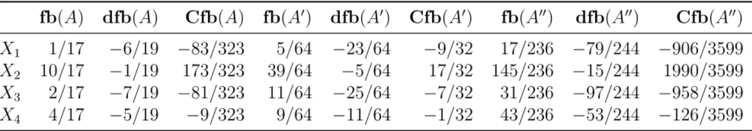
Proposition 5.7. Copeland fair bets methods violate RCS on the set RR. Figure 8: Ranking problems of Example 8
(a) Ranking problem (N, A) X1
X2
X3 X4
(b) Ranking problem (N, A0) X1
X2
X3 X4
Proof.
Example 8. Let (N, A) ∈ R and (N, A0) ∈ R be the ranking problems in Figure 8 with the set of objects N ={X1, X2, X3, X4} and tournament matrices
A=
0 0 1 0
1 0 1 0.5
0 0 0 1
1 0.5 0 0
and A0 =
0 0 0.5 0.5
1 0 0.5 1
0.5 0.5 0 0
0.5 0 1 0
with the same matches matrix
M =
0 1 1 1 1 0 1 1 1 1 0 1 1 1 1 0
.
Let (N, A00) = (N, A+A0)∈ RR be the sum of these two ranking problems.
The rating vectors are given in Table 6: Cf b1(N, A)< Cf b3(N, A) andCf b1(N, A0)<
Cf b3(N, A0), but Cf b1(N, A00)> Cf b3(N, A00).
Table 6: Fair bets and associated rating vectors of Example 8
fb(A) dfb(A) Cfb(A) fb(A0) dfb(A0) Cfb(A0) fb(A00) dfb(A00) Cfb(A00) X1 1/17 −6/19 −83/323 5/64 −23/64 −9/32 17/236 −79/244 −906/3599 X2 10/17 −1/19 173/323 39/64 −5/64 17/32 145/236 −15/244 1990/3599 X3 2/17 −7/19 −81/323 11/64 −25/64 −7/32 31/236 −97/244 −958/3599 X4 4/17 −5/19 −9/323 9/64 −11/64 −1/32 43/236 −53/244 −126/3599
6 Additivity and irrelevant comparisons
Definition 6.1. Independence of irrelevant matches (IIM): Let (N, R, M) ∈ R be a ranking problem and Xi, Xj, Xk, X` ∈ N be four different objects. Let f : R → Rn be a scoring procedure such that fi(N, R, M)≥fj(N, R, M) and (N, R0, M)∈ R be a ranking problem identical to (N, R, M) except for the result r0k` 6=rk`. f is called independent of irrelevant matches if fi(N, R0, M)≥fj(N, R0, M).
IIM means that all comparisons not involving the chosen objects are irrelevant from the perspective of their relative ranking. It appears asindependence in Rubinstein (1980, Axiom III) and Nitzan and Rubinstein (1981, Axiom 5) for round-robin ranking problems.
The name independence of irrelevant matches was introduced by Gonz´alez-D´ıaz et al.
(2014), however, they also allowed for a change in the number of matches between two objects (i.e. a0k` 6=ak` implies that possibly both r0k` 6=rk` and m0k` 6=mk`), which seems to be too general for us. Altman and Tennenholtz (2008, Definition 8.4) introduces a still stronger axiom called Arrow’s independence of irrelevant alternatives by permitting modifications of comparisons involving Xi and Xj if rih−rih0 = rjh −r0jh holds for all Xh ∈N \ {Xi, Xj}.
Remark 6. Property IIM has a meaning if n≥4.
Sequential application of independence of irrelevant matches can result in a ranking problem (N, R0, M) ∈ R, for which rgh0 = rgh if {Xg, Xh} ∩ {Xi, Xj} 6= ∅, but all other paired comparisons are arbitrary.
Lemma 6.1. The score method satisfies IIM.
Proposition 6.1. The generalised row sum, least squares, fair bets, dual fair bets and Copeland fair bets methods violate IIM.
Proof.
Example 9. Let (N, R, M) ∈ R and (N, R0, M) ∈ R be the ranking problems in Figure 9 with set of objects N ={X1, X2, X3, X4} and tournament matrices
A =
0 0.5 0 0.5 0.5 0 0.5 0
0 0.5 0 0
0.5 0 1 0
and A0 =
0 0.5 0 0.5 0.5 0 0.5 0
0 0.5 0 1
0.5 0 0 0
,
where a0346=a34.
Figure 9: Ranking problems of Example 9 (a) Ranking problem (N, R, M)
X1
X2
X3 X4
(b) Ranking problem (N, R0, M) X1
X2
X3 X4
IIM requires that f1(N, R, M) ≥ f2(N, R, M) ⇔ f1(N, R0, M) ≥ f2(N, R0, M). Let x(ε)(N, R, M) = x(ε), x(ε)(N, R0, M0) = x(ε)0 and q(N, R, M) = q, q(N, R0, M0) = q0. Here
x1(ε) =x2(ε)0 = (1 +εmn) ε
(1 + 2ε)(1 + 4ε) = ε
1 + 2ε and x1(ε)0 =x2(ε) = (1 +εmn) −ε
(1 + 2ε)(1 + 4ε) = −ε 1 + 2ε, that is, X1 x(ε)(N,R,M) X2 but X1 ≺x(ε)(N,R0,M) X2.
Regarding the least squares method, on the basis of Lemma 2.2:
q1 = limε→∞x1(ε)
mn =q20 = limε→∞x2(ε)0
mn = 1
2 · 1 4 = 1
8 and q10 = limε→∞x1(ε)0
mn =q2 = limε→∞x2(ε) mn =−1
2 ·1 4 =−1
8. Hence X1 q(N,R,M) X2 but X1 ≺q(N,R0,M)X2.
Table 7: Fair bets and associated rating vectors of Example 9
fb(N, A) dfb(N, A) Cfb(N, A) fb(N, A0) dfb(N, A0) Cfb(N, A0) X1 5/16 −3/16 1/8 3/16 −5/16 −1/8 X2 3/16 −5/16 −1/8 5/16 −3/16 1/8 X3 1/16 −7/16 −3/8 7/16 −1/16 3/8 X4 7/16 −1/16 3/8 1/16 −7/16 −3/8 The other three rating vectors are given in Table 7. Thus f b1(N, A) > f b2(N, A), df b1(N, A) > df b2(N, A) and Cf b1(N, A) > Cf b2(N, A), but f b1(N, A0) < f b2(N, A0), df b1(N, A0)< df b2(N, A0) and Cf b1(N, A0)< Cf b2(N, A0), which is a contradiction.
Remark 7. In Example 9, the two ranking problems coincide with the permutation σ(X1) = X2 and σ(X3) = X4. Therefore independence of irrelevant matches demands thatf1(N, R, M) =f2(N, R, M), which is violated by all ranking methods discussed except for the score.
Lemma 6.2. The generalised row sum and least squares methods satisfy IIM on the set RR.
Proof. Due to the axiomsagreement (Chebotarev, 1994, Property 3) andscore consistency (Gonz´alez-D´ıaz et al., 2014), both the generalised row sum and least squares methods coincide with the score on this set of problems, so Lemma 6.1 holds.
Proposition 6.2. Fair bets, dual fair bets and Copeland fair bets methods violate IIM on the set RR.
Figure 10: Ranking problems of Example 10 (a) Ranking problem (N, A)
X1
X2
X3 X4
(b) Ranking problem (N, A0) X1
X2
X3 X4
Proof.
Example 10. Let (N, A)∈ R and(N, A0)∈ R be the ranking problems in Figure 10 with the set of objects N ={X1, X2, X3, X4} and tournament matrices
A =
0 1 0 0.5
0 0 0.5 1
1 0.5 0 0
0.5 0 1 0
and A0 =
0 1 0 0.5
0 0 0.5 1
1 0.5 0 1
0.5 0 0 0
,
where a0346=a34.
Table 8: Fair bets and associated rating vectors of Example 10
fb(N, A) dfb(N, A) Cfb(N, A) fb(N, A0) dfb(N, A0) Cfb(N, A0)
X1 1/4 −1/4 0 5/32 −7/32 −1/16
X2 1/4 −1/4 0 7/32 −5/32 1/16
X3 1/4 −1/4 0 19/32 −1/32 9/16
X4 1/4 −1/4 0 1/32 −19/32 −9/16
IIM requires that f1(N, R, M) ≥ f2(N, R, M) ⇔f1(N, R0, M) ≥ f2(N, R0, M). The rating vectors are given in Table 8. Thusf b1(N, A)≥f b2(N, A),df b1(N, A)≥df b2(N, A) and Cf b1(N, A) ≥ Cf b2(N, A), but f b1(N, A0) < f b2(N, A0), df b1(N, A0) < df b2(N, A0) and Cf b1(N, A0)< Cf b2(N, A0), which is a contradiction.
Gonz´alez-D´ıaz et al. (2014, p. 165) consider independence of irrelevant matches a drawback of the score method because outside the subdomain of round-robin ranking problems, it makes sense for the scoring procedure to be responsive to the strength of the opponents.
Our discussion is finalized by linkingIIM to additivity.