Dynamic Modeling and Simulation of a Switched Reluctance Motor in a Series Hybrid Electric Vehicle

Dynamic Modeling and Simulation of a

Switched Reluctance Motor in a Series Hybrid Electric Vehicle

Siavash Sadeghi, Mojtaba Mirsalim

Department of Electrical Engineering Amirkabir University of Technology Tehran, Iran

E-mail: sadegs3@rpi.edu, mirsalim@aut.ac.ir

Arash Hassanpour Isfahani

Islamic Azad University, Khomeinishar Branch Isfahan, Iran

Email: ahassanpour@ieee.org

Abstract: Dynamic behavior analysis of electric motors is required in order to accurately evaluate the performance, energy consumption and pollution level of hybrid electric vehicles. Simulation tools for hybrid electric vehicles are divided into steady state and dynamic models. Tools with steady-state models are useful for system-level analysis whereas tools that utilize dynamic models give in-depth information about the behavior of sublevel components. For the accurate prediction of hybrid electric vehicle performance, dynamic modeling of the motor and other components is necessary. Whereas the switched reluctance machine is well suited for electric and hybrid electric vehicles, due to the simple and rugged construction, low cost, and ability to operate over a wide speed range at constant power, in this paper dynamic performance of the switched reluctance motor for e series hybrid electric vehicles is investigated. For this purpose a switched reluctance motor with its electrical drive is modeld and simulated first, and then the other components of a series hybrid electric vehicle, such as battery, generator, internal combusion engine, and gearbox, are designed and linked with the electric motor. Finally a typical series hybrid electric vehicle is simulated for different drive cycles. The extensive simulation results show the dynamic performance of SRM, battery, fuel consumption, and emissions.

Keywords: Dynamic Modeling, Switched Reluctance Motor, Series Hybrid Electric Vehicle, ADVISOR, Vehicle Performance

1 Introduction

Environmental and economical issues are the major driving forces in the development of electric vehicles (EVs) and hybrid electric vehicles (HEVs) for urban transportation. The selection of the right electric motor is of primary importance to the EVs and HEVs designer [1]. Several types of electrical machines, such as DC, induction, and permanent magnet machines, have been used for HEV applications [1, 2, 3, 4]. These days switched reluctance motors (SRM) have become more attractive for these applications due to the simple and rugged construction, low cost, and ability to operate over a wide speed range at constant power [5].

Several computer programs have since been developed to simulate and analyze HEVs. The advanced vehicle simulator (ADVISOR) is the most widely used computer simulation tool. The structure of ADVISOR makes it ideal for interchanging a variety of components, vehicle configurations, and control strategies. Also, the capability to quickly perform parametric and sensitivity studies for specific vehicles is a unique and invaluable feature of ADVISOR [6, 7]. However, this software only models the steady-state mode, and one cannot see the dynamic performance of electric motors in the simulation. Furthermore, the model for a SRM hasn't been included in the software library of ADVISOR yet [6, 7]. Since the dynamic behavior analysis of electric machines is required in order to accurately evaluate the performance, energy consumption and pollution level of HEVs, it is necessary to model the electric machine dynamically.

Among the various types of HEVs, series hybrid electric vehicles (SHEVs) attract special attention due to their simple structure and uncomplicated energy management strategy. As there is no mechanical connection between the internal combustion engine (ICE) and load, the engine speed and torque is completely independent of vehicle load. Therefore, the engine can run in its optimal efficiency region all the time and minimize engine emissions [8]. In this paper, a co- simulation method is implemented to dynamically model and simulate SHEVs.

For this purpose, utilizing MATLAB/SIMULINK software, dynamic modeling of a switched reluctance motor is investigated and simulated separately. In doing so, mechanical components of a SHEV are also called from the software library of ADVISOR and then linked with the electric motor. Finally a typical SHEV is modeled and simulated for different drive cycles using the proposed method. The extensive simulation results show the dynamic performance of SRM, battery, fuel consumption, and emissions for the drive cycle.

2 Vehicle Performance

The first step in vehicle performance modeling is to obtain an equation for calculating the required vehicle propelling force. This force must overcome the road load and accelerate the vehicle. The tractive force, Ftot, available from the propulsion system can be written as [9, 10]:

tot roll AD grade acc

F = f + f +f + f (1)

The rolling resistance, aerodynamic drag, and climbing resistance are known as the road load. The rolling resistance is due to the friction of the vehicle tires on the road and can be written as [9, 10]:

roll r

f = f ⋅M g⋅ (2)

where,M ,f_r and g are the vehicle mass, rolling resistance coefficient and gravity acceleration, respectively.

The aerodynamic drag is due to the friction of the vehicle body moving through the air. The formula for this component is [9, 10]:

1 2

AD 2 D

f = ⋅ ⋅ξ C ⋅ ⋅A V (3)

where,V , ξ, C_D and Aare the vehicle speed, air mass density, aerodynamic coefficient and the frontal area of the vehicle, respectively.

The climbing resistance is due to the slope of the road and is expressed by [9, 10]:

grade sin

f =M g⋅ ⋅ α (4)

where, α is the angle of the slope.

If the velocity of the vehicle is changing, then clearly a force will be needed to be applied in addition to the above forces. This force will provide the linear acceleration of the vehicle, and is given by:

acc

f M a M dV

= ⋅ = ⋅ dt (5)

A typical road load characteristic as a function of vehicle speed and vehicle mass is shown in Fig. 1.

Wheels and axle convert F_totand the vehicle speed to torque and angular speed requirement to the differential as follows:

wheel

wheel tot wheel wheel Loss

T F R I d T

dt

= ⋅ + ⋅ ω + (6)

(

)

wheel wheel

V s

ω = R + (7)

where T_wheel, R_wheel, I_wheel, T_Loss, ω_wheel, and s are the tractive torque, radius of the wheel, wheel inertia, wheel loss torque, angular velocity of the wheels and wheel slip wheels, respectively.

The torque at the wheels and the wheel angular velocity are converted to engine torque and engine speed requirements using the gears ratio at differential and gearbox as in the following:

0 50

100 150 600

800 1000 1200200

400 600 800 1000

Vehicle speed(Km/h) Vehicle mass(Kg)

Road load force(N)

Figure 1

The road load profile as a function of vehicle speed and vehicle mass (α =0 deg.)

_ _ _ _

_ _ _

1

1

gb

fd in gb out fd out fd Loss fd

fd

engine

engine gb in gb out gb Loss gb

gb

T T T T I d

dt G

T T T T I d

dt G ω ω

⎛ ⎞

= =⎜ + + ⋅ ⎟

⎝ ⎠

⎛ ⎞

= =⎜ + + ⋅ ⎟

⎝ ⎠

(8)

gb fd wheel

engine gb gb

G G

ω ω

ω ω

= ⋅

= ⋅ (9)

where the subscripts fdand gb stand for differential and gear box and T_{fd_in},

( )

_

fd out wheel

T =T , T_{fd_Loss}, I_fd, G_fd, T_engine, ω_gb and ω_engine, are the input and output differential torques, differential loss torque, differential inertia, differential gear, engine torque, gearbox and engine angular velocities, respectively.

3 Components Modeling of a Series Hybrid Vehicle

In addition to design studies of overall hybrid power-train systems that tend to use relatively simple models for vehicle components, the authors have looked into the integration of system simulations with high-fidelity component models, such as models of motors, and engines.

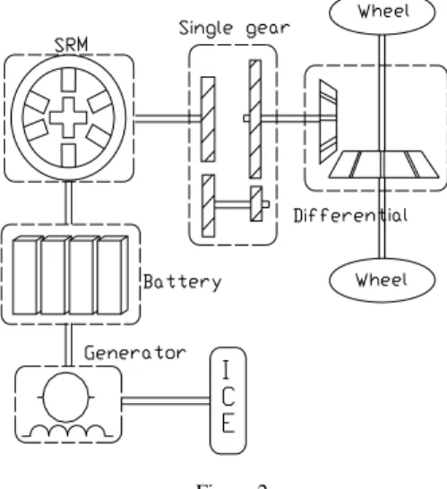
The structure of a series hybrid vehicle shown in Fig. 2 consists of two major groups of components:

1) Mechanical components (Wheels and Axle, Transmission box and ICE).

2) Electrical components (battery, electric motor and generator).

Figure 2 The model for a SHEV

3.1 Transmission Box

In SHEVs the differential box can be eliminated by using two electric motors.

Because of the wide speed range operation of electric motors enabled by power electronics control, it is possible for SHEVs to use a single gear ratio for instantaneous matching of the available motor torque (T_m) with the desired tractive torque (T_wheel). The single gear ratio and its size will depend on the maximum motor speed, maximum vehicle speed, and the wheel radius as in the following [11]:

( )

max m

fd gb wheel

GR G G R

V

= ⋅ = ω ⋅ (10)

where

( )

3.2 Battery

The NiMH type battery is selected for the system and the complex battery model reported in [8] is simplified and used in the simulations. This model can be described by an equivalent circuit which consists of an open circuit voltage,V_oc, in series with an internal resistance,R_int varying with the state of charge (SOC). The relation betweenV_oc,R_int, SOC, and temperature can be easily obtained from the data available from the battery manufacturer, or simple experimental tests. The voltage of the battery tends to drop as the SOC decreases and as the amount of current drawn from the battery increases.

SOC can be calculated from the maximum capacity of the battery as in the following:

(

)

Soc= Capacity −Ah Capacity

3600

batt used

Ah =

∫

where Ah and I_batt stand for Ampere-hour and the current, respectively. The terminal voltage of the battery,V_batt, can be determined as follows:

int

batt oc batt

V =V −R ⋅I (12)

It is apparent that during the motoring phase of a drive cycle, the electric machine draws current from the battery pack (discharging) and in the regenerative braking mode the machine supplies current to the pack (charging).

3.3 Electric Machine

One important component that can be introduced in greater detail is the electric machine. Electric machines are the key components of SHEVs. Some motor types have inherent property of operation with large extended speeds. The direct current motor is an example, but it has low efficiency, a high need of maintenance and low reliability due to the presence of the commutators. An induction motor (IM) can achieve a large speed range with field-oriented control. However, due to nonlinearity of the dynamic IM model and the dependency on motor parameters, the control is complex [5]. A permanent magnet motor (PM) has the highest torque density and therefore will potentially have the lowest weight for given torque and power ratings [10, 12]. However, the fixed amount of flux for magnets

limits its extended speed range. An SRM has certain advantages, such as rugged construction, fault-tolerant operation, and low cost, which makes it well suited with many applications such as vehicle propulsion. Design and simulation shows a wide speed range of 5.7 (and 6.7 times the based speed), much higher than other kinds of electric motors [10]. Therefore, it can be considered an excellent candidate for SHEVs. In this paper the dynamic model of an SRM is investigated in a series hybrid vehicle.

The model of an SRM is described by its flux linkage and torque characteristics.

Some approaches have been used to obtain these characteristics from finite element (FE) analysis to complex nonlinear magnetic circuit models [13]. Since FE analysis is time consuming, in this paper an analytical model is used to model the flux linkage and torque characteristics. In the analytical method, the flux linkage is described with an analytical equation in two positions: unaligned position and poles overlap position. Then, the current can be calculated as in the following [13]:

ph

ph ph ph

V d i R

dt

= λ + (13)

ph ph ph ph

ph

d di d

dt i dt dt

λ λ λ θ

θ

∂ ∂

= ⋅ + ⋅

∂ ∂ (14)

1

ph ph

ph ph ph

ph ph

di V i R

dt i

λ ω

λ θ

⎛ ∂ ⎞

=∂ ∂ ⎜⎝ − − ∂ ⎟⎠ (15)

where:

ph d ph

dt BEMF

λ θ ω λ

θ θ

∂ ∂

⋅ = ⋅ =

∂ ∂

The phase torque in SRM is obtained from the co-energy method which can be calculated from the phase flux linkage as follows:

0

( , )

( , )

i ph

ph

T W i θ i di

λ θ

θ θ

∂ ′ ∂

= =

∂ ∂

∫

The total electromagnetic torque is obtained by:

1

( , )

q

total phase j j

j

T T i θ

=

=

∑

where q is number of phases.

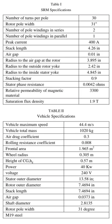
Fig. 3 illustrates the phase static torque versus different phase currents and rotor positions for an SRM with parameters given in Tables I-II.

Table I SRM Specifications

Number of turns per pole 30

Rotor pole width 31^o

Number of pole windings in series 2 Number of pole windings in parallel 1

Peak current 400 A

Stack length 4.26 in

Air gap 0.01 in

Radius to the air gap at the rotor 3.895 in Radius to the outside rotor yoke 2.42 in Radius to the inside stator yoke 4.845 in

Stacking factor 0.9

Stator phase resistance 0.0042 ohms Relative permeability of magnetic

material

3300 Saturation flux density 1.9 T

TABLEII Vehicle Specifications

Vehicle maximum speed 44.4 m/s Vehicle total mass 1020 kg Air drag coefficient 0.3 Rolling resistance coefficient 0.008

Frontal area 1.965 m²

Wheel radius 0.305 m

Height of CG,hg 0.57 m

Power 40 Kw

voltage 240 V

Stator outer diameter 13.58 in;

Rotor outer diameter 7.4694 in

Stack length 7.4694 in

Air gap 0.0373 in

Shaft diameter 2.8135

Rotor pole width 31 degree M19 steel

-50 -40 -30 -20 -10 0 10 20 30 40 50 -300

-200 -100 0 100 200 300

θ(degree)

Phase torque(N.m)

54A108A 162A216A 270A

Figure 3

Phase static torque versus rotor position at different phase currents

The most flexible and versatile four-quadrant SRM converter is the bridge converter as shown in Fig. 4, which requires two switches and two diodes per phase. The switches and diodes must be rated to withstand the supply voltage plus any transient overload. Here in the circuit, an IGBT switch is used because of its high input impedance as in a MOSFET, and low conduction losses similar to BJTs [14]. This circuit is capable of operating the machine as a motor and a generator.

Ph2 Ph3 Vbus Ph1

+

_

Figure 4 Converter topology

3.4 SRM Controller

The speed controller for an SRM is the same as for other electric motors and can be shown with a PI controller. However, the torque control is important for this motor and is different from other electric motors. In the torque control of a switched reluctance machine, the torque command is executed by regulating the current, as shown in Fig. 5. The control method alters for different speeds of the motor. Below the base speed, the torque is controlled by the pulse width

modulation (PWM) control of current where the phase voltage is switched between zero and Vbus (soft-chopping). Above the base speed with constant power, due to the high back electromotive force (BEMF), which cannot be field weakened, PWM control of current is not possible. Fig. 6 shows the BEMF of the SRM for different speeds. Operation in constant power is made possible in this motor by the phase advancing of the stator phase current, until overlapping between the successive phases occurs [15, 16]. Therefore, the torque of the SRM is controlled with current chopping or PWM control of current under the base speed, and with the phase turn-on and turn-off angles above the base speed. The control of the SRM in generating mode is identical to motoring mode. The only difference is the timing of current pulses. In motoring mode, the windings are excited during the rise of inductance (approaching of poles), while in generating mode each winding is excited when the poles separate from each other. At lower speeds, the current pulses are controlled by chopping the voltage between zero and -Vbus with fixed commutation angles. At higher speeds the generator is operated in single-pulse mode [15, 16].

Speed Controller

Torque Controller

Angle Calculator

Current

Controller Converter SRM

T_ref I_ref

Gate Signals ωref

ω θ

θon θ_off

Tload

Figure 5 SRM Controller drive

-50 -40 -30 -20 -10 0 10 20 30 40 50 -600

-400 -200 0 200 400 600

θ(degree)

BEMF(V)

N=5100rpm N=4100rpm N=3100rpm N=2100rpm N=1100rpm

N=100rpm

Figure 6

BEMF voltage of an SRM versus rotor position at different speeds (Iph=150A)

Figs. 7 and 8 show the SRM characteristics in low speed motoring and generating modes, respectively. Since the speed is low, control of the motor is done by chopping the phase current around the reference current. The power supply current is positive and shows that the motor is absorbing energy from the battery in an electric propulsion system. In the generating mode, the power supply current is negative; therefore the machine is supplying energy to charge the battery. It is seen from Fig. 9 that the SRM current cannot be chopped completely due to the high back EMF at high speeds, and thus, control of the motor is done by the phase advancing of the stator phase current. Fig. 10 illustrates the SRM torque and power versus motor speed.

0 1 2 3

0 200 400

600 ^(a)

t(s)

N(rpm)

3 3.05 3.1

-200 0 200

400 ^(b)

t(s)

Torque(N.m)

3.03 3.04 3.05 3.06 -400

-200 0 200 400

(c)

t(s)

Voltage&Current(V,A)

3 3.05 3.1

-500 0 500 1000

(d)

t(s)

iL(A)

Figure 7

SRM characteristics for ωref=500rpm T, load=200 .N m

0 1 2 3 0

500 1000

(a)

t(s)

N(rpm)

3 3.05 3.1

-300 -200 -100 0

100 ^(b)

t(s)

Torque(N.m)

3.03 3.04

-400 -200 0 200

400 ^(c)

t(s)

Voltage&Current(V,A)

3 3.05 3.1

-400 -200 0 200

400 ^(d)

t(s)

iL(A)

Figure 8

SRM characteristics for ωref=500rpm T, load= −200 .N m

0 1 2 3

0 2000 4000 6000 8000

t(s)

N(rpm)

(a)

3.49 3.495 3.5

-100 0 100 200

t(s)

Torque(N.m)

(b)

3.49 3.495 3.5

-400 -200 0 200 400

t(s)

Voltage&Current(V,A)

(c)

3.49 3.495 3.5

-100 0 100 200 300

t(s)

iL(A)

(d)

Figure 9

SRM characteristics for ω_ref=6000rpm T, _load=50 .N m

0 2500 5000 7500 100000 50

100 150 200 250

N(rpm)

T(N.m)

0 0 2500 5000 7500 10000 1

2 3 4x 10⁴

N(rpm)

P(watt)

Figure 10

SRM torque and power versus speed

3.5 Generator

The model for the generator is chosen from the library in ADVISOR. This model is unidirectional; i.e. it has one input (the applied torque to the shaft and the rpm), and one output (electrical power output from the generator). From the characteristics of efficiency versus revolution per minute (rpm) and torque, and by the use of a look-up table, the model is able to calculate the output power of the generator and the energy losses at any instant.

3.6 ICE

The model of the internal combustion engine is also chosen from the ADVISOR.

The input and output of the model are the desired torque and speed and the developed torque and speed, respectively. If the developed torque and speed are within the operating limits and are obtainable at the specified time step, then the response values are exactly equal to the desired values. In addition to dynamic calculations, the model for the ICE can predict important quantities such as fuel consumption and the amounts of air pollutants in the simulation. This model includes the effects of the inertia of the ICE on operation and the operational boundaries of the engine, and also the effects of temperature on fuel consumption and the pollutants. The modeling of an ICE is complicated, and by the use of engine maps the complexity is reduced to some extant.

The governing output torque and speed equations, or in other words, the desired quantities for the gearbox, are written as in the following:

_ _

engine out MAP engine engine

engine out MAP

T T I α

ω ω

= − ⋅

= (18)

where, α_engine, I_engine, T_MAP and ω_MAPare the acceleration and the inertia of the ICE, and the torque and speed determined from the engine maps, respectively.

The fuel consumption and the amount of pollutants are stored in tables indexed by fuel converter speed and torque. The primary output of the exhaust system model is the tailpipe emissions (HC, CO, NOx, and PM) in g/s, as a function of time.

Other outputs include the temperature of various exhaust system components and of the exhaust gas temperature into and out of each system component.

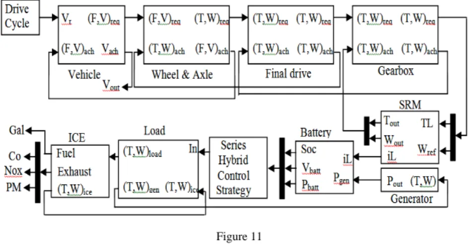
4 Linking between the Components and the Control method of SHEVs

The integration of the models of different electrical and mechanical components, where each block consists of two groups of inputs and two groups of the desired outputs, is shown in Fig. 11. One can see that the modeling of each block is a feed-backward.

Figure 11 SHEV Model

As for the control strategy of a hybrid vehicle, once again the ADVISOR software is implemented. The main strategy of the control system in a series hybrid is to keep the level of charge of the batteries at a specified range, while charging the batteries at maximum efficiency. In this research, the following control scheme is implemented:

• If the SOC of batteries goes below a specified level, the ICE is turned on to supply energy to the motor and the batteries via an electric generator.

• If the ICE is already turned on, it must stay on till the SOC reaches a high specified level, and as soon the level is reached, the ICE is turned off.

• While staying turned on, the ICE must operate at its maximum efficiency point (best operating point).

5 Simulation Results

Simulation results presented here focus on the dynamic behavior of SRM and the battery of the vehicle. The system is simulated for a 12% road slope on the ECE+EUDC test cycle. The cycle is used for emission certification of light duty vehicles in Europe. Due to dynamic modeling of the electric motor in SIMULINK, the mentioned drive cycle requires about 25 hours of simulation time on a computer with a Pentium 4 processor and 512 MB of memory. The data for the SRM and EV is in the Appendix. The SRM used in the simulation is rated at 240 V and 40 kW. Now, the required number of modules of 12- volt NiMH batteries with the Voc, and Rint values shown versus SOC in Fig.12 would be twenty.

Since the SRM used in this simulation has a maximum speed of 8000 rpm, the single gear ratio can be calculated from (10) as follows:

( )

max

8000 2

60 0.305 5.75 44.4

m

wheel

GR r

V

ω ^⎛⎜_⎝ ^⋅ π^⎞⎟_⎠

= ⋅ = ⋅ ≈

0 0.2 0.4 0.6 0.8 1

0.005 0.01 0.015 0.02 0.025

Soc

Rint(ohm)

0 0.2 0.4 0.6 0.8 1

12.5 13 13.5 14 14.5

Soc

Voc(V)

Figure 12 Voc and Rint versus SOC

The dynamic behaviors of the SHEV in the ECE+EUDC+12% drive cycle (Fig.

13) are shown in Figs. 14 to 20. The SRM reference and real speeds are shown in Figs. 16 and 17. The SRM load torque and developed torque are also shown in Figs. 16 and 17. It can be seen from Fig. 15 that the torque ripple has no significant effect on the motor speed. The vehicle reference and real speeds are depicted in Fig. 18. Figs. 19 and 20 show the performance of the battery, i.e., the current versus time. The Figure shows the negative SRM current which can be returned to the battery and which therefore increases the overall efficiency of the vehicle.

0 100 200 300 400 500 0

10 20 30 40 50

time(sec)

V(Km/h)

Figure 13

ECE-EUDC Drive cycle ( with 12% slope)

0 100 200 300 400 500

0 50 100 150 200 250

time(sec) ω(rad/s)

Figure 14 SRM reference speed

0 100 200 300 400 500

-50 0 50 100 150 200 250

time(sec)

ω(rad/s)

Figure 15 SRM actual speed

0 100 200 300 400 500 -20

0 20 40 60 80 100

time(sec)

T(N.m)

Figure 16 SRM load torque

0 100 200 300 400 500

-50 0 50 100 150 200 250

time(sec)

T(N.m)

Figure 17 SRM torque

0 100 200 300 400 500

0 10 20 30 40 50

time(sec)

V(Km/h)

mesure ref.

Figure 18 Vehicle speed and drive cycle

0 100 200 300 400 500 -400

-200 0 200 400

time(sec)

iL(A)

Figure 19 Battery current

0 100 200 300 400 500

0.6 0.62 0.64 0.66 0.68 0.7 0.72

time(sec)

Soc

Figure 20 State of charge

Fuel consumption, the state of charge of batteries, and the level of exhaust emissions for the mentioned drive cycle are investigated in Figs. 21 to 24. In these figures, the drive cycle repeats for 15 times and the state of battery charge is kept between 0.4 and 0.7. The rate of pollution caused by ICE is high at the beginning of ICE work period because the engine is still cold. However, the amounts of pollutants decrease as the motor becomes warm enough. The total amount of exhaust emissions for 15 repetitions of the cycle is shown in Fig. 23. The variation of output voltage of battery is as seen in Fig. 24.

0 2000 4000 6000 8000 0

1 2 3 4

time(sec)

Fuel(L)

Figure 21 Fuel consumption

0 2000 4000 6000 8000

0.4 0.5 0.6 0.7 0.8

time(sec)

Soc

Figure 22 State of charge

0 50 100 150 200

Gram(g)

Nox

Co

Hc

Figure 23 Exhaust output

0 2000 4000 6000 8000 160

180 200 220 240 260 280 300

time(sec)

Battery voltage(V)

vbus voc

Figure 24 Battery voltage

Conclusions

A co-simulation method has been implemented to dynamically model and simulate the performance of a switch reluctance motor integrated into SHEVs. For this purpose, utilizing MATLAB/SIMULINK software, a dynamic model of a switched reluctance motor has been implemented. A close loop control system with PI controller is employed to control the speed of the motor. The mechanical components of a SHEV are then called from the software library of ADVISOR and then linked with the switch reluctance motor drive in MATLAB/SIMULINK.

To evaluate the dynamic performance of switch reluctance motor drive, a typical SHEV has been modeled and simulated for an ECE+EUDC drive cycle with 12%

of road slope. The extensive simulation results show the proper dynamic performance of SRM, battery, fuel consumption, and emissions for drive cycles.

References

[1] M. Ehsani, Yimin Gao, S. Gay, "Characterization of Electric Motor Drives for Traction Applications," in proc. 29^th IEEE Industrial Electronics Society Annual Conference, IECON’03, Nov. 2-6, 2003, Volume 1, pp. 891- 896 [2] M. Zeraoulia et al, “Electric Motor Drive Selection Issues for HEV

Propulsion Systems: A Comparative Study,” IEEE Trans. Vehicular Tech., Vol. 55, pp. 1756-1763, Nov. 2006

[3] L. Chang, "Comparison of AC Drives for Electric Vehicles - A report on Experts' Opinion Survey," IEEE AES Systems Magz. pp. 7-10, Aug. 1994 [4] Z. Preitl, P. Bauer, J. Bokor, “Cascade Control Solution for Traction Motor

for Hybrid Electric Vehicles”, Acta Polytechnica Hungarica, Journal of Applied Sciences at Budapest Tech, Hungary, Vol. 4, Issue 3, pp. 75-88, 2007

[5] K. M. Rahman, B. Fahimi, G. Suresh, A. V. Rajarathnam, M. Ehsani,

"Advantages of Switched Reluctance Motor Applications to EV and HEV:

Design and Control Issues", IEEE Trans. on Industry Applications, Vol. 36, No. 1, Jan./Feb., 2000, pp. 111-121

[6] T. Markel, A. Brooker, T. Hendricks, V. Johnson, K. Kelly, B. Kramer, M.

O' Keefe, S. Sprik, K. Wipke, "ADVISOR: a Systems Analysis Tool for Advanced Vehicle Modeling", ELSEVIER Journal of Power Sources, Vol.

110, pp. 255-266, 2002

[7] M. Amrhein, P. T. Krein,” Dynamic Simulation for Analysis of Hybrid Electric Vehicle System and Subsystem Interactions, Including Power Electronics,” IEEE Trans. on Vehicular Technology, Vol. 54, No. 3, May 2005

[8] S. Barsali, C. Miulli, A. Possenti, "A Control Strategy to Minimize Fuel Consumption of Series Hybrid Electric Vehicles", IEEE Trans. on Energy Conversion, Vol. 19, No. 1, March 2004

[9] James Larminie, John Lowry, Electric Vehicle Technology Explained, John Wiley, England, 2003

[10] M. Ehsani, Y. Gao, S. Gay, A. Emadi, Modern Electric, Hybrid Electric, and Fuel Cell Vehicles, CRC press, USA, 2005

[11] K. M. Rahman, H. A. Toliyat, M. Ehsani, "Propulsion System Design of Electric and Hybrid Vehicles," IEEE Trans. on Industrial Electronics, Vol.

44, No. 1, pp. 19-27, Feb. 1997

[12] C. C. Chen, K. T. Chau, Modern Electric Vehicle Technology, Published by the US by Oxford University Press, Inc., New York, 2001, pp. 122-133 [13] A. V. Radun, "Design Considerations for the Switched Reluctance Motor,"

IEEE Trans. on Industry Applications, Vol. 31, No. 5, Sep. 1995

[14] I. Husain, M. S. Islam, "Design, Modeling and Simulation of an Electric Vehicle System," SAE Technical Paper Series. 1999-01-1149

[15] Do-Hyun Jang, "The Converter Topology with Half Bridge Inverter for Switched Reluctance Motor Drive," ISIE Conference, Pusan, Korea, 2001 [16] T. J. E. Miller, Switched Reluctance Motors and their Control. Lebanon,

Ohio: Magna Physics Publishing, 1993

[17] A. V. Radun, "Generating with the Switched Reluctance Motor,"

Proceedings of the Ninth Annual Applied Power Electronics Conference and Exposition, Vol. 1, p. 41, 1994