Számítás intelligencia alapú regressziós technikák és alkalmazásaik a folyamatmérnökségben

PhD Thesis

KENESEI TAMÁS

PANNON EGYETEM 2014.

DOI: 10.18136/PE.2014.563

Számítási intelligencia alapú regressziós technikák és alkalmazásaik a folyamatmérnökségben

Értekezés doktori (PhD) fokozat elnyerése érdekében a

Pannon Egyetem Vegyészmérnöki Tudományok és Anyagtudományok Doktori Iskolájához tartozóan

Írta:

Kenesei Tamás Péter Konzulens: Dr. Abonyi János

Elfogadásra javaslom (igen/nem) ...

(aláírás) A jelölt a doktori szigorlaton ... %-ot ért el.

Az értekezés bírálóként elfogadásra javaslom:

Bíráló neve: igen/nem ...

(aláírás) Bíráló neve: igen/nem ...

(aláírás)

A jelölt az értekezés nyilvános vitáján ...%-ot ért el.

Veszprém, ...

a Bíráló Bizottság elnöke A doktori (PhD) oklevél min˝osítése ...

...

az EDT elnöke

Pannon Egyetem

Vegyészmérnöki és Folyamatmérnöki Intézet Folyamatmérnöki Intézeti Tanszék

Számítási intelligencia alapú regressziós

technikák és alkalmazásaik a folyamatmérnökségben

DOKTORI (PhD) ÉRTEKEZÉS Kenesei Tamás

Konzulens

Dr. habil. Abonyi János, egyetemi tanár

Vegyészmérnöki és Anyagtudományok Doktori Iskola

2014.

University of Pannonia

Institute of Chemical and Process Engineering Department of Process Engineering

Computational Intelligence based regression techniques and their applications in process engineering

PhD Thesis Tamás Kenesei

Supervisor

János Abonyi, PhD, full professor

Doctoral School in Chemical Engineering and Material Sciences

2014.

Köszönetnyilvánítás

Mindazoknak akik hittek bennem.

"Együtt hajtunk, együtt halunk, rossz fiúk t˝uzön–vízen át!"

Kivonat

Számítási intelligencia alapú regressziós technikák és alkal- mazásaik a folyamatmérnökségben

Az olyan adat alapú regressziós modellek mint a metsz˝o hipersíkok, neurális hálózatok vagy szupport vektor gépek széles körben elterjedtek a szabályzásban, optimalizálásban és a folyamat monitorozásban. Mivel ezek a modellek nem értel- mezhet˝oek, a folyamatmérnökök gyakran nem a legjobb gyakorlat szerint hasznosítják ezeket. Abban az esetben, ha betekintést nyerhetnénk ezekbe a fekete doboz mod- ellekbe, lehet˝oségünk nyílna a modellek validálására, további információk és össze- függések feltárására a folyamat változok között, illetve a modell építés fázisát is tudnánk támogatni a-priori információk beépítésével.

Az értekezés kulcs gondolata, hogy a metsz˝o hipersíkok, neurális hálózatok és szupport vektor gépek fuzzy modellekké alakíthatóak, és a kapott szabálybázis alapú rendszerek értelmezése biztosítható speciális modell redukciós és vizualizá- ciós technikákkal.

Az értekezés els˝o harmada a metsz˝o hipersík alapú regressziós fák identifiká- ciójával foglakozik. A m˝uködési tartomány rekurzívan particionált egy fuzzy c- regresszió alapú csoportosítási technikával. A kapott kompakt regressziós fa lokális lineáris modellekb˝ol áll. Ez a modellezési struktúra jól használható modell alapú szabályozásban, például modell prediktív szabályozás során.

A következ˝o fejezet a neurális hálózatok validálásával, vizualizálásával és struk- turális redukciójával foglalkozik, melyek alapjául a neurális hálózat rejtett rétegének fuzzy szabálybázissá történ˝o átalakítása szolgál.

Végül a szupport vektor gépek és a fuzzy modellek közti analógia kerül betu- tatásra egy 3 lépéses redukciós algoritmus segítségével. A cél értelmezehet˝o fuzzy regressziós modell, melynek alapja a szupport vektor regresszió.

A fejlesztett algoritmusok vegyészmérnöki gyakorlatban történ˝o alkalmazható- ságát minden fejezetben esettanulmányok igazolják.

Abstract

Computational intelligence based regression techniques and their applications in process engineering

Data-driven regression models like hinging hyperplanes, neural networks and support vector machines are widely applied in control, optimization and process monitoring. Process engineers are often mistrustful of the application of these mod- els since they are not interpretable. If we would have some insight to these black boxes we could have the possibility to validate these models, extract hidden infor- mation about the relationships among the process variables, and to support model identification by incorporating some prior knowledge.

The key idea of this thesis is that hinging hyperplanes, neural networks and sup- port vector machines can be transformed into fuzzy models and the interpretability of the resulted rule-base systems can be ensured by special model reduction and visualization techniques.

The first part of the thesis deals with the identification of hinging hyperplane based regression trees. The operating regime of the model is recursively partitioned by a novel fuzzy c-regression clustering based technique. The resulted compact regression tree consists of local linear models, which model structure is favored in model based control solutions, like in model predictive control.

The next section deals with the validation, visualization and structural reduction of neural networks based on the transformation of the hidden layer of the network into an additive fuzzy rule base system.

Finally, based on the analogy of support vector regression and fuzzy models a three-step model reduction algorithm will be proposed to get interpretable fuzzy regression models on the basis of support vector regression.

Real life utilization of the developed algorithms is shown by sectionwise exam- ples taken from the area of process engineering.

Contents

1 Introduction 1

1.1 Data-driven techniques in process engineering . . . 1

1.2 Interpretability and model structure identification . . . 4

1.3 Computational intelligence based models . . . 6

1.4 Motivation and outline of the thesis . . . 9

2 Hinging Hyperplanes 12 2.1 Identification of hinging hyperplanes . . . 14

2.1.1 Hinging hyperplanes . . . 14

2.1.2 Improvements in hinging hyperplane identification . . . 17

2.2 Hinging hyperplane based binary trees . . . 22

2.3 Application examples . . . 26

2.3.1 Benchmark data . . . 26

2.3.2 Dynamic systems . . . 28

Identification of the Box-Jenkins gas furnace . . . 28

Model predictive control . . . 30

2.4 Conclusions . . . 37

3 Neural Networks 38 3.1 Structure of Neural Networks . . . 38

3.1.1 McCulloch-Pitts neuron . . . 39

3.2 NN Transformation into Rule Based Model . . . 41

3.2.1 Rule–based interpretation of neural networks . . . 41

3.3 Model Complexity Reduction . . . 44

3.4 NN Visualization Methods . . . 45

3.5 Application Examples . . . 47

3.5.1 pH process . . . 47

3.5.2 pH dependent structural relationship model for capillary zone electrophoresis of tripeptides . . . 51

3.6 Conclusions . . . 52

4 Support Vector Machines 53 4.1 FIS interpeted SVR . . . 55

4.1.1 Support Vector Regression Models . . . 55

4.1.2 Structure of Fuzzy Rule-based regression model . . . 57

4.2 Ensuring interpretability with three–step algorithm . . . 58

4.2.1 Model Simplification by Reduced Set Method . . . 58

4.2.2 Reducing the Number of Fuzzy Sets . . . 60

4.2.3 Reducing the Number of Rules by Orthogonal Transforms . 61 4.3 Application Examples . . . 62

4.3.1 Illustrative example . . . 62

4.3.2 Identification of Hammerstein System . . . 62

4.4 Conclusions . . . 64

5 Summary 66 5.1 Introduction . . . 66

5.2 New Scientific Results . . . 67

5.3 Utilization of Results . . . 69

5.4. Bevezetés . . . 70

5.5. Új tudományos eredmények . . . 71

5.6. Az eredmények gyakorlati hasznosítása . . . 73

Appendices 79

A Introduction to regression problems 79

B n–fold cross validation 82

C Orthogonal least squares 84

D Model of the pH Process 86

E Model of electrical water heater 88

List of Figures

1.1 Steps of the knowledge discovery process . . . 3

1.2 Tradeoffs in modeling . . . 4

1.3 Model complexity versus modeling error . . . 5

1.4 Framework of the thesis . . . 9

2.1 Basic hinging hyperplane definitions . . . 15

2.2 Hinging hyperplane identification restrictions . . . 19

2.3 Hinging hyperplane model with 4 local constraints and two parameters 21 2.4 Hinging hyperplane based regression tree for basic data sample in case of greedy algorithm . . . 23

2.5 Modeling a 3D function with hinging hyperplane hyperplane based tree . . . 25

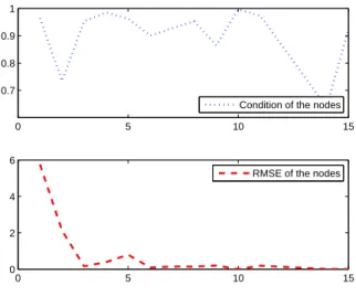
2.6 Node by nodeϱand RMSE results for non–greedy tree building . . 26

2.7 Node by nodeϱand RMSE results for greedy tree building . . . 26

2.8 Identification of the Box–Jenkins gas furnace model with hinging hyperplanes . . . 29

2.9 The water heater . . . 30

2.10 Free run simulation of the water heater (proposed hinging hyper- plane model, neural network, linear model) . . . 31

2.11 Structure of the MPC controller . . . 32

2.12 Performance of the MPC based on linear model . . . 35

2.13 Performance of the MPC based on Neural Network model . . . 35

2.14 Performance of the MPC based on hinging hyperplane . . . 36

3.1 A biological neuron and its model (McCulloch-Pitts neuron) . . . . 39

3.2 Modeling framework . . . 40

3.3 Interactive or operator . . . 42

3.4 Interpretation of the activation function . . . 43 3.5 Similarity index . . . 46 3.6 Decomposed univariate membership functions . . . 48 3.7 Distances between neurons mapped into two dimensions with mds . 49 3.8 Error reduction ratios . . . 49 4.1 Illustrative example with model output, support vectors and the in-

sensitive region . . . 63 4.2 Hammerstein system . . . 63 4.3 Identified Hammerstein system, support vectors and model output

after reduction . . . 64 4.4 Non-distinguishable membership functions obtained after the appli-

cation of RS method . . . 64 4.5 Interpetable membership functions of the reduced fuzzy model . . . 65 D.1 Scheme of the pH setup. . . 86 E.1 The scheme of the physical system. . . 88

List of Tables

1.1 Evaluation criteria system . . . 7

2.1 Comparison of RMSE results of different algorithms. (Numbers in brackets are the number of models) . . . 27

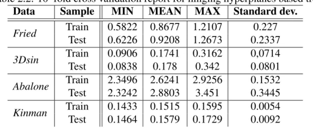
2.2 10–fold cross validation report for hinging hyperplanes based tree . 28 2.3 RMSE results of the generated models . . . 29

2.4 RMSE results of the generated models . . . 32

2.5 Simulation results (SSE - sum squared tracking error, CE - sum square of the control actions) . . . 36

3.1 One-step ahead prediction results. . . 48

3.2 Training errors for different model structures and model reductions. (Number of neurons in the hidden layer of the network/Number of reduced neurons from the given model structure) . . . 50

3.3 One-step ahead prediction results. . . 51

4.1 Results on Regress data . . . 62

4.2 Results on Hammerstein system identification . . . 63

A.1 Functions with the ability to transform them to linear forms . . . 81

D.1 Parameters used in the simulations. . . 87

E.1 Parameters used in the simulation model of the heating system. . . . 89

Abbreviations

ANN Artificial Neural Network APC Advanced process control CSTR Continuous stirred tank reactor

FIS Fuzzy system

FCRM Fuzzy c–regression clustering method

DT Decision tree

FAS Fuzzy additive system LOLIMOT Locally linear model tree

KDD Knowledge data discovery in databases HH Hinging hyperplanes

PDFS Positive definite fuzzy system SVM Support vector machine SVR Support vector regression

NARX Nonlinear Autoregressive with eXogenous Input

NN Neural Network

MDS Multi-dimensional scaling MLP Multilayer perceptron MPC Model predictive control RBF Radial basis function

RS Reduced set method

RMSE Root main square error OLS Orthogonal least squares TS Takagi-Sugeno fuzzy model

Notations

Regression problem x independent variable y dependent variable θ model parameter ρ cardinality Fuzzy logic

δ rule consequent

µ_i,k membership value, whereistands for the clusters and k for the data points (k = 1. . . n).

Λ a priori constraints v cluster center

U fuzzy partition matrix Dynamic systems

E, J cost function n_a output order n_b input order α filter value

Q(u) cartridge heater performance Q_M maximum power

u heating signal T_out outlet temperature H_p prediction horizon Hc control horizon λ weighting coefficient α filter parameter

Neural networks and support vector machines β firing strenght

τ bias

ϕ feature mapping S similarity measure k kernel function

∗ interactive oroperator ε error tolerance

ξ_i, ξ_i^∗ slack variables C cost coefficient

Ni input space dimension N_x number of support vectors N_R reduced set expansion

Chapter 1

Introduction

With combination of computation intelligence tools, like hinging hyperplanes (HH), support vector regression (SVR), artificial neural networks (ANNs) and fuzzy mod- els powerful and interpretable models can be developed. This introduction presents the motivation of handling these techniques in one integrated framework and de- scribes the structure of the thesis.

1.1 Data-driven techniques in process engineering

Information for process modeling and identification can be obtained from different sources. According to the type of available information, three basic levels of model synthesis are defined:

White-box or first-principle modeling A complete mechanistic model is const- ructed from a priori knowledge and physical insight. Here dynamic models are derived based on mass, energy and momentum balances of the process [1].

Fuzzy logic modeling A linguistically interpretable rule-based model is formed based on the available expert knowledge and measured data [1].

Black-box model or empirical model No physical insight is available or used, but the chosen model structure belongs to families that are known to have good flexibility and have been "successful in the past". Model parameters are iden- tified based on measurement data [1].

This means, if we have good mechanistic knowledge about the process, this can be transformed into white box model described by analytical (differential) equa-

tions. If we have information like human experience described by linguistic rules and variables, the mechanistic modeling approach is useless and the application of rule-based approaches like fuzzy logic is more appropriate [2, 3]. Finally, there may be situations, where the most valuable information comes from input-output data collected during operation. In this case, the application of black box models is the best choice. These black box models are especially valuable, when an accu- rate model of the process dynamics is needed. Therefore, the nonlinear black box modeling is a challenging and promising research field [4, 5, 6, 7, 8].

Black-box models are especially valuable when an accurate model of the pro- cess dynamics is needed. In order to perform a successful data-driven model the following steps have to be carried out [1]:

1. Selection of model structure and complexity 2. Design of exctitation signals used or identification 3. Identification of model parameters

4. Model validation

Process engineers are often mistrustful of the application of nonlinear black box models since they are not interpretable. If we would have some insight to these black boxes we could have the possibility to validate these models, extract hidden information about the relationships among the process variables, selection of the model structure based on this knowledge, and to support model identification by incorporating some prior knowledge.

For these purposes novel model identification methods, interpretable, robust and transparent models are needed. Since we are interested in extraction of knowledge from process data, tools and methodologies of data mining should be also efficiently utilized.

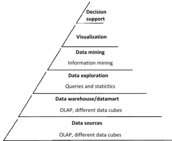
Historically the notion of finding useful patterns in data has been given a variety of names including data mining, knowledge extraction, information discovery, and data pattern processing. The term data mining has been mostly used by statisti- cians, data analysts, and the management information systems (MIS) communities [9]. Data mining is not just a simple tool, but a complex process consisting of mul- tiple steps, hence this process must be integrated into the supported activity. The process of data–based knowledge discovery can be seen on Fig. 1.1. Introducing the knowledge discovery process allows us to give a brief definition to data mining:

Data mining is a decision support process to give valid, useful and a priori not known reliable information from data sources.[10]

Decision support

Queries and statictics

OLAP, different data cubes Information mining

Data sources Visualization Data mining

Data exploration

Data warehouse/datamart

OLAP, different data cubes

Figure 1.1: Steps of the knowledge discovery process

To understand this definition the following keywords must be further investi- gated [1]:

process Data mining is not a product–ready delivered software generating auto- matically consumable knowledge from stored data, but it is a complex pro- cess consisting of well–defined steps. Regression techniques takes place dur- ing model preparation. Improved model identification algorithms and inter- pretable models ensure quality of acquired information at the end of KDD process.

valid Mined information must be accurate and statistically significant. Validity states not only accuracy but also completeness.

useful It is not enough to generate valid knowledge with the help of data mining, explored knowledge must be utilizable for the exactly defined problem. Un- fortunately measuring usefulness is not always solved, as sometimes affect of the used information cannot be measured with monetary tools.

preliminarily not known Strictly speaking, data–based knowledge discovery has twofold aim: confirmation and discovery. Confirmation means strengthen- ing hypothesis of the data expert while discovery stands for identification of patterns generated by the examined system. Aim of data mining basically is

to identify discoverable knowledge to define predictive or descriptive func- tions. Regression–based methods are predictive exercises defining future, not known properties or behaviors of the modeled process.

exact Result of data mining must be easily interpretable, and the model should not deviate from from reality.

Key challenge of data mining is to capture potential information from opaque data sources and transform data to a more compact, abstract, informative and easy- to-use way. Hence, data mining looks for trends and patterns in large databases.

Knowledge delivered by data mining exists in a form of an interpretable model or information represented in decision trees, rule bases, networks or mathematical equations.

The aim of the thesis at hand is to extract interpretable regression models to foster the usage of these models in process engineering.

1.2 Interpretability and model structure identifica- tion

Interpretability

Maintenance

Complexity Reliability

1 100

1 100

1

Figure 1.2: Tradeoffs in modeling

Zadeh stated in Principle of Incompatibility [11] "as the complexity of a system increases our ability to make precise and yet significant statements about its behav- ior diminishes until a threshold is reached beyond which precision and significance (or relevance) become almost mutually exclusive characteristics." Obtaining high degree of interpretability with sizeable complexity is a contradictory purpose and - in practice - one of these properties prevails over the other. The problem becomes

much more difficult to handle when model reliability and maintenance is included to the conditions.

In most studies of process identification it is assumed that there is an opti- mal functional structure describing relationship between measured input and output data. It is very difficult to find a functional structure for a nonlinear system. Gen- erally speaking, the structure identification of a system has to solve two problems:

one is to find input variables and one is to find input-output relations. The selection the input variables can be based on the aim of the modeling exercise and on prior knowledge related to the system to be modeled. For static systems statistical tech- niques, correlation analysis and modeling performance based methods proposed by Sugeno [12, 13, 14] and Jang [15] can be used. For dynamical systems, the selec- tion of the relevant model-inputs is identical to the determination of the model order of the NARX model.

The identified model must be validated as well. If the model is validated by the same data set from which it was estimated, the accuracy of the model always improves as the complexity of the model structure increases. In practice, a trade- off is usually sought between model accuracy and complexity, and there are several approaches to compensate for this automatic increase of the modeling performance.

Fig. 1.3 shows connection between modeling error and model complexity[1].

As this figure shows, selection of the proper model structure is a complex tasks that requires careful selection of training and validation datasets, proper cost functions and proper optimization strategies or heuristics that support the modeler.

Large Modell complexity

train set

test set

Small

Prediction error

Figure 1.3: Model complexity versus modeling error

1.3 Computational intelligence based models

Majority of problems arose in process engineering practice requires data-driven modeling of nonlinear relationships between experimental and technological vari- ables. Complexity of nonlinear regression techniques is gradually expanding with the development of analytical and experimental techniques, hence model structure and parameter identification is a current and important topic in the field of nonlinear regression not just by scientific but also from industrial point of view as well.

In line with these expectations and taking interpretability of regression models as basic requirement aim of this thesis is the development of robust computational intelligence models in order to solve nonlinear regression identification tasks.

Tools from the armory of computational intelligence (also referred as soft com- puting) have been in focus of researches recently, since soft computing techniques are used for fault detection, forecasting of time-series data, inference, hypothesis testing, and modeling of causal relationships (regression techniques) in process en- gineering.

The meaning of soft computing was originally tailored in the early 1990s by Dr. Zadeh [16]. Soft computing refers to a collection of computational techniques in computer science, artificial intelligence, machine learning and some engineering disciplines, to solve two cardinal problems:

• Learning from experimental data (examples, samples, measurements, records, patterns) by neural networks and support vector based techniques

• Embedding existing structured human knowledge(experience, expertise, heuris- tic) into fuzzy models [17]

These approaches attempt to study, model, and analyze very complex phenom- ena: those for which more conventional methods have not yielded low cost, analytic, and complete solutions. Earlier computational approaches (hard computing) could model and precisely analyze only relatively simple systems.

As more complex systems arising in biology, medicine, the humanities, manage- ment sciences, and similar fields often remained intractable to conventional math- ematical and analytical methods. Where hard computing schemes –striving for ex- actness and full truth–fail to render the given problem, soft computing techniques deliver robust, efficient and optimal solutions to capture available design knowledge for further analysis.

Generally speaking, soft computing techniques resemble biological processes more closely than traditional techniques, which are largely based on formal logical systems, such as sentential logic and predicate logic, or rely heavily on computer- aided numerical analysis. Hence in real life high degree of uncertainty should be taken in to account during identification process. Soft computing tries to solve this challenge with exploiting tolerance for imprecision, uncertainty and partial truth in order to reach robustness and transparency at low cost.

Many systems are not amenable to conventional modeling approaches due to the lack of precise, formal knowledge about the system, due to strongly nonlinear be- havior, high degree of uncertainty, or time-varying characteristics. Computational intelligence, the technical umbrella of hinging hyperplanes (HH) [18, 19, 20], sup- port vector regression (SVR) [21, 22, 23, 24, 25], artificial neural networks (ANNs) [26, 27, 28, 29, 30, 31] and fuzzy logic [2, 3, 32] has been recognized as a powerful tool which is tolerant of imprecision and uncertainty, and can facilitate the effective development of models by combining information from different sources, such as first-principle models, heuristics and data.

Table 1.1: Evaluation criteria system

Property Description

Interpolation behavior Character of the model

output between training data samples Extrapolation behavior Character of the model

outside region of training data

Locality Locality, globality

of the basis functions

Accuracy Model accuracy

with given number of parameters Smoothness Smoothness of model output Sensitivity to noise Affect of noise on model behavior Parameter optimization Can linear and nonlinear

model parameters estimated Structure optimization Possibilities of model

structure and complexity optimization Online adaptation Possibilities of on-line model adaptable Training speed Speed of model parameter estimation Evaluation speed Speed of model evaluation

Curse of dimensionality Model scale up to higher input space dimensions Interpretation Interpretation of model

parameters and model structure Incorporation of constraints Difficulty of constraint incorporation

Usage Acceptability and penetration of modeling structure

Among the techniques of computational intelligence, ANNs attempt to mimic the structures and processes of biological neural systems. They provide powerful analysis properties such as complex processing of large input/output information arrays, representing complicated nonlinear associations among data, and the ability to generalize or form concepts-theory. Support vector regression in it’s nature is very similar to ANNs and on the other hand HH models can be a good alternative to NNs.

Based on [1] Table 1.1 summarizes several criterion can be used to evaluate these modeling techniques. The studied nonlinear regression techniques have usu- ally robust modeling structure, however the resulted model is often a non–inter- pretable black–box model. This thesis focuses on the identification, utilization and interpretability of ANNs, HHs and SVR in the realm of modeling, identification and control of nonlinear processes.

1.4 Motivation and outline of the thesis

This thesis has twofold aims to introduce new algorithms for nonlinear regression (hinging hyperplanes) and to highlight possibilities to transform black–box non- linear regression models (neural networks and support vector regression) to trans- parent and interpretable fuzzy rule base (see fig 1.4). These techniques together form a framework to utilize combination-of-tools-methods in order to understand, visualize and validate non–linear black box models.

Neural Network Models

Support Vector Regression Hinging hyperplanes

Fuzzy Logic

Figure 1.4: Framework of the thesis

Three algorithms were examined based on the evaluation criteria system men- tioned in section 1.2 in details namely identification of regression trees based hing- ing hyperplane, neural networks and support vector regression. Application of these techniques eventuate black box models at first step. It will be shown how inter- pretability could be maintained during model identification with utilization of ap- plicable visualization and model structure reduction techniques within the fuzzy modeling framework.

Chapter 2 Hinging hyperplanes deals with the identification of hinging hyper- plane based regression trees. Results of the developed algorithm proves that the im- plementation of a priori constraints enables fuzzy c-regression clustering technique to identify hinging hyperplane models. Application of this technique recursively on the partitioned input space ends up in a regression tree capable for modeling and even for implementation of model predictive control of technological data coming from real life applications. According to the evaluation system mentioned in section 1.2 the development algorithm contains major developments in hinge model identi- fication, since the proposed method has higher accuracy, the tree–based represen- tation enables betterstructureandparameter optimizationand helpsinterpretation of model parameters and model structure.

Main improvements of hinging hyperplane identification is discussed in

T. Kenesei, B. Feil, J. Abonyi, Fuzzy Clustering for the Identification of Hinging Hyperplanes Based RegressionLecture notes in computer science, Lecture notes in artificial intelligence; 4578. ISBN:9783540733997 pp. 179-186. 2007

Detailed description of regression tree representation can be found in

T. Kenesei, J. Abonyi, Hinging hyperplane based Regression tree identified by Fuzzy Clustering WSC16 - 16th Online World Conference on Soft Computing in Industrial Applications2011.

Hinging hyperplane model predictive control is published in

T. Kenesei, B. Feil, J. Abonyi, Identification of Dynamic Systems by Hinging Hy- perplane ModelsICAI 2007 - 7th International Conference on Applied Informatics Eger 2007.

Our efforts within the framework of hinging hyperplane identification and control is submitted to

T. Kenesei, J. Abonyi, Hinging hyperplane based Regression tree identified by Fuzzy Clustering and its application Applied Soft Computing Journal vol 13(2) pp. 782-792 2013.

Chapter 3 Visualization and reduction of neural networksdeals with the vali- dation, visualization and structural reduction of neural networks in order to achieve betterinterpretability. With applying orthogonal least squares and similarity mea- sure based techniques structure optimization is also performed. It is described in details that the hidden layer of the neural network can be transformed to an additive fuzzy rule base.

Reduction and visualization methods are described in

T. Kenesei, B. Feil, J. Abonyi, Visualization and Complexity Reduction of Neural Networks Applications of soft computing: updating the state of art., pp. 43-52.

2009. Advances in soft computing ISBN:9783540880783vol. 52.

Chapter 4 Interpretable Support vector regression describes connections be- tween fuzzy regression and support vector regression, and introduces a three-step reduction algorithm to get interpretable fuzzy regression models on the basis of sup- port vector regression. This combination–of–tools technique retains goodgeneral-

izationbehavior and noiseinsensitivenessof the support vector regression however keeps the identified modelinterpretableand with the application of reduction tech- niquesstructure optimizationis also achieved.

Three-step reduction algorithm and visualization methods can be found in

T. Kenesei, A. Roubos, J. Abonyi, A Combination-of-Tools Method for Learning Interpretable Fuzzy Rule-Based Classifiers from Support Vector MachinesLecture Notes in Computer Science; 4881. ISBN:978-3-540-77225-5pp. 477-486. 2008 Application of support vector regression models is described in the following pub- lications

T. Kenesei, J. Abonyi, Interpretable Support Vector Machines in Regression and Classification- Application in Process Engineering, Hungarian Journal of Indus- trial Chemistry, VOL 35. pp. 101-108 2007.

T. Kenesei, J. Abonyi, Interpretable Support Vector Regression, Artificial Intelli- gence Research, Vol 1 (2), ISSN:1927-6974 ,2012

Real life utilization of the developed algorithms is shown by section–wise exam- ples taken from the area of chemical engineering. Finally, Chapter 5 summarizes the new scientific results in English and in Hungarian.

The proposed framework supports the structure and parameter identification of regression models. To achieve this goal structure optimization techniques like or- thogonal least squares (OLS) and decision tree based model representations are applied. The detailed description of the regression problem are given in Appendix A while OLS is described in details in Appendix C.

As can be seen, this thesis is based on a number of papers we published recently.

I have attempted to eliminate redundancy of these papers. To promote easier reading consistent nomenclature list can be found in the Notations section. Source codes of the utilized softwares written in Matlab can be found on the www.abonyilab.com website.

Chapter 2

Hinging Hyperplanes

Hinging hyperplane model is proposed by Breiman [20] and identification of this type of non-linear model is several times reported in the literature due to suffer- ing from convergency and range problems [33, 34, 35, 19]. Methods like penalty of hinging angle were proposed to improve Breiman’s algorithm [18], or Gauss–

Newton algorithm can be used to obtain the final non–linear model [34]. Several application examples have been also published in the literature, e.g. it can be used in identification of piecewise affine systems via mixed-integer programming [36]

and this model also lends himself to form hierarchical models [19].

In this chapter a much more applicable algorithm is proposed for hinging hyper- plane identification. The key idea is that in a special case (c= 2) fuzzy c-regression method (FCRM) [37] can be used for identifying hinging hyperplane models. To ensure that two local linear models used by fuzzy c-regression algorithm form a hinging hyperplane function, it has to be granted that local models are intersecting each other in the operating regime of the model. The proposed constrained FCRM algorithm is able to identify one hinging hyperplane model, therefore to generate more complex regression trees, described method should be recursively applied.

Hinging hyperplane models containing two linear submodels divide operating re- gion of the model into two parts, since hinging hyperplane functions define a linear separating function in the input space of the hinging hyperplane function. Sequence of these separations result a regression tree where branches correspond to linear di- vision of operating regime based on the hinge of the hyperplanes at a given node.

This type of partitioning can be considered as crisp version of a fuzzy regression based tree described in [38]. Fortunately, in case of hinging hyperplane based re- gression tree there is no need for selecting best splitting variable at a given node, but on the other hand it is not as interpretable as regression trees utilizing univariate

decisions at nodes.

The proposed modeling framework is based on the algorithm presented at the 16th Online Conference on Soft Computing in Industrial Applications [39]. To support the analysis and building of this special model structure novel model performance and complexity measures are presented in this work. Special attention is given for the modeling and controlling nonlinear dynamical systems. Therefore, application example related to Box–Jenkins gas furnace benchmark identification problem is added. It will be also shown that thanks to the piecewise linear model structure the resulted regression tree can be easily utilized in model predictive control. A detailed application example related to the model predictive control of a water heater will demonstrate the benefits of the proposed framework.

A critical step in the application of model-based control is the development of a suitable model for the process dynamics. This difficulty stems from lack of knowl- edge or understanding of the process to be controlled. Fuzzy modeling has been proven to be effective for the approximation of uncertain nonlinear processes. Re- cently, nonlinear black-box techniques using fuzzy and neuro-fuzzy modeling have received a great deal of attention [40]. Readers interested in industrial applications can find an excellent overview in [41]. Details of model-based control relevant ap- plications are well presented in [42] and [43].

Most nonlinear identification methods are based on the NARX (Nonlinear AutoRe- gressive with eXogenous input) model [8]. The use of NARX black box models for high-order dynamic processes in same cases are impractical. Data–driven iden- tification techniques alone, may yield unrealistic NARX models in terms of steady- state characteristics, local behavior and unreliable parameter values. Moreover, the identified model can exhibit regimes which are not found in the original system [43]. This is typically due to insufficient information content of the identification data and the over-parametrization of the model. This problem can be remedied by incorporating prior knowledge into the identification method by constraining the parameters of the model [44]. Another possibility to reduce the effects of over- parametrization is to restrict the structure of the NARX model, using for instance the Nonlinear Additive AutoRegressive with eXogenous input (NAARX) model [45]. In this thesis a different approach is proposed, a hierarchial set of local linear models are identified to handle complex systems dynamics.

Operating regime based modeling is a widely applied technique for identification of these nonlinear systems. There are two approaches for building operating regime based models. An additive model uses sum of certain basis functions to represent a

non-linear system, while partitioning approach partitions the input space recursively to increase modeling accuracy locally [18]. Models generated by this approach are often represented by trees [46]. Piecewise linear systems [47] can be easily repre- sented in a regression tree structure [48]. Special type of regression tree is called locally linear model tree, which algorithm combines a heuristic strategy for input space decomposition with a local linear least squares optimization (like LOLIMOT [1]). These models are hierarchical models consisting of nodes and branches. Inter- nal nodes represent tests on input variables of the model, and branches correspond to outcomes of said tests. Leaf (terminal) nodes contains regression models in case of regression trees.

Thanks to the structured representation of the local linear models, hinging hyper- planes lend themselves to a straightforward incorporation in model based control schemes. In this chapter this beneficial property is demonstrated in the design of instantaneous linearization based model predictive control algorithm [32].

This chapter organized as follows: next section discusses how hinging hyperplane functions’ approximation is done with FCRM identification approach. The descrip- tion of tree growing algorithm and the measures proposed to support model building are given in Section 2.2. In Section 4.3, application examples are presented while Section 4.4 concludes the chapter.

2.1 Identification of hinging hyperplanes

2.1.1 Hinging hyperplanes

The following section gives a brief description about the hinging hyperplane ap- proach on the basis of [34, 18, 49], followed by how the constrains can be incor- porated into FCRM clustering.

For a sufficiently smooth functionf(x_k), which can be linear or non-linear, assum- ing that regression data{xk, yk}is available fork = 1, . . . , N. Functionf(xk)can be represented as the sum of a series of hinging hyperplane functions h_i(x_k), i = 1,2, . . . , K are defined as the hinging hyperplane function. Breiman[20] proved that we can use hinging hyperplane to approximate continuous functions on com- pact sets, guaranteeing a bounded approximation error

∥e_n∥=∥f−

∑K i=1

h_i(x)∥ ≤(2R)⁴c²/K (2.1)

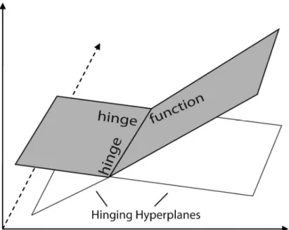
Figure 2.1: Basic hinging hyperplane definitions

where K is the number of hinging hyperplane functions R is the radius of the sphere in which the compact set is contained and c is such that

∫

∥w∥²|f(w)|dw =c <∞ (2.2) The approximation with hinging hyperplane functions can get arbitrarily close if sufficiently large number of hinging hyperplane functions are used. The sum of the hinging hyperplane functions∑K

i=1h_i(x_k)constitutes a continuous piecewise linear function. The number of input variablesnin each hinging hyperplane function and the number in hinging hyperlane functions K are two variables to be determined.

The explicit form for representing a functionf(x_k)with hinging hyperplane func- tions becomes (see Fig. 2.1)

f(x_k) =

∑K i=1

h_i(x_k) =

∑K i=1

⟨max|min⟩(

x^T_kθ_1,i,x^T_kθ_2,i)

(2.3) where⟨max|min⟩means max or min.

Suppose two hyperplanes are given by:

y_k=x^T_kθ₁, y_k =x^T_kθ₂ (2.4)

wherexk = [xk,0, xk,1, xk,2, . . . , xk,n],xk,0 ≡1is thekth regressor vector andyk

is thekth output variable. These two hyperplanes are continuously joined together at {x : x^T (θ₁−θ₂) = 0} as can be seen in Fig. 2.1. As a result they are called hinging hyperplanes. The joint△ =θ₁−θ₂, multiples of△are definedhingefor the two hyperplanes,yk = x^T_kθ1 andyk =x^T_kθ2. The solid/shaded part of the two hyperplanes explicitly given by

y_k = max(x^T_kθ₁,x^T_kθ₂)ory_k = min(x^T_kθ₁,x^T_kθ₂) (2.5) Hinging hyperplane method has some interesting advantages for non-linear function approximation and identification:

1. Hinging hyperplanes functions could be located by a simple computation- ally efficient method. In fact hinging hyperplane models are piecewise linear models, the linear models are usually obtained by repeated use of linear least- squares method, which is very efficient. The aim is to improve the whole identification method with more sophisticated ideas.

2. For non–linear functions with resemble hinging hyperplane functions, the hinging hyperplane method has very good and fast convergence properties.

Hinging hyperplane method practically combines some advantages of neural networks (in particular ability to handle very large dimensional inputs) and of con- structive wavelet based estimators (availability of very fast training algorithms).

Essential hinging hyperplane search problem can be viewed as an extension of linear least-squares regression problem. Linear least-squares regression aims to find the best parameter vector bθ, by minimizing a quadratic cost function with which regression model gives the best linear approximation toy. For nonsingular data matrixX linear least squares estimatey = x^Tθ is always uniquely available.

The hinging hyperplane search problem, on the other hand, aims to find the two parameter vectorsθ1 andθ2, defined by

[θ1, θ2] = arg min

θ1,θ2

∑N k=1

[⟨max|min⟩(

yk−x^T_kθ1, yk−x^T_kθ2

)]2

(2.6) A brute force application of Gauss-Newton method can solve the above de- scribed optimization problem. However, two problems exist [18]:

1. High computational requirement. The Gauss–Newton method is computa- tionally intensive. In addition, since the cost function is not continuously

differentiable, the gradients required by Gauss-Newton method can not be given analytically. Numerical evaluation is thus needed which has high com- putational demand.

2. Local minima. There is no guarantee that the global minimum can be ob- tained. Therefore appropriate initial condition is crucial.

2.1.2 Improvements in hinging hyperplane identification

The proposed identification algorithm applies a much simpler optimization method, the so–called alternating optimization which is a heuristic optimization technique and has been applied for several decades for many purposes, therefore it is an ex- haustively tested method in non–linear parameter and structure identification as well. Within the hinging hyperplane function approximation approach, the two linear submodels can be identified by the weighted linear least-squares approach, but their operating regimes (where they are valid) are still an open question.

For that purpose fuzzyc-regression model (further referred as FRCM and proposed by Hathaway and Bezdek [37]) was used. This technique is able to partition the data and determine the parameters of the linear submodels simultaneously. With the application of alternating optimization technique and taking advantage of the linearity in(y_k−x^T_kθ₁)and(y_k−x^T_kθ₂), an effective approach is given for hinging hyperplane function identification, hence FCRM method in a special case (c = 2) is able to identify hinging hyperplanes. The proposed procedure is attractive in lo- cal minima point of view as well, because in this way although the problem is not avoided but transformed into a deeply discussed problem, namely the cluster valid- ity problem.

The following quadratic cost function can be applied for the FCRM method

E_m(U,{θ_i}) =

∑c i=1

∑N k=1

(µ_i,k)^mE_i,k(θ_i) (2.7)

wherem∈ ⟨1,∞)denotes a weighting exponent which determines the fuzziness of the resulting clusters, whileθ_i represents the parameters of local models andµ_i,k ∈ Uis the membership degree, which could be interpreted as a weight representing the extent to which the value predicted by the model f_i(x_k, θ_i) matches y_k. The

prediction error is defined by:

Ei,k =(

yk−fi(xk;θi))2

(2.8) but other measures can be applied as well, provided they fulfill the minimizer prop- erty stated by Hathaway and Bezdek [37].

One possible approach to the minimization of the objective function (2.7) is the group coordinate minimization method that results in the following algorithm:

• InitializationGiven a set of data {(x₁, y₁), . . . ,(x_N, y_N)}spec- ify c, the structure of the regression models (2.8) and the error measure (2.7). Choose a weighting exponentm > 1and a termi- nation toleranceϵ >0. Initialize the partition matrix randomly.

• RepeatForl= 1,2, . . .

Step 1 Calculate values for the model parameters θ_i that minimize the cost functionE_m(U,{θ_i}).

Step 2 Update the partition matrix µ^(l)_i,k = 1

∑c

j=1(E_i,k/E_j,k)^2/(m−1), 1≤i≤c, 1≤k ≤N (2.9) until||U^(l)−U^(l−1)||< ϵ.

A specific situation arises when the regression functionsf_i are linear in the param- etersθ_i, f_i(x_k;θ_i) = x^T_i,kθ_i, wherex_i,k is a known arbitrary function ofx_k. In this case, the parameters can be obtained as a solution of a set of weighted least-squares problem where the membership degrees of the fuzzy partition matrixUserve as the weights.

The N data pairs and the membership degrees are arranged in the following matrices.

X =







 x^T_i,1 x^T_i,2 ... x^T_i,N







 , y=







 y₁ y₂ ... y_N









, Φ_i =









µ_i,1 0 · · · 0 0 µ_i,2 · · · 0 ... ... . .. ... 0 0 · · · µ_i,N









(2.10)

The optimal parametersθ_i are then computed by:

θi = [X^TΦiX]⁻¹X^TΦiy (2.11) Applying c = 2 during FCRM identification these models can be used as base identifiers for hinging hyperplane functions. For hinging hyperplane function iden-

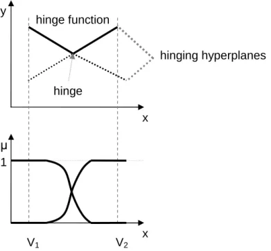
hinging hyperplanes hinge function

hinge

x

x y

µ 1

V₁ V₂

Figure 2.2: Hinging hyperplane identification restrictions

tification purposes, two prototypes have to be used by FCRM (c = 2), and these prototypes must be linear regression models. However, these linear submodels have to intersect each other within the operating regime covered by the known data points (within the hypercube expanded by the data). This is a crucial problem in the hing- ing hyperplane identification area [18]. To take into account this point of view as well, constrains have to be taken into consideration as follows. Cluster centers vi can also be computed from the result of FCRM as the weighted average of the known input data points

v_i =

∑N

k=1x_kµ_i,k

∑_N

k=1µ_i,k (2.12)

where the membership degreeµi,k is interpreted as a weight representing the extent to which the value predicted by the model matches y_k. These cluster centers are located in the ’middle’ of the operating regime of the two linear submodels. Because the two hyperplanes must cross each other following criteria can be specified (see

Fig. 2.9):

v1(θ1−θ2)<0 and v2(θ1−θ2)>0or (2.13) v₁(θ₁−θ₂)>0 and v₂(θ₁−θ₂)<0

These relative constrains can be used to take into account the constrains above:

Λ_rel,1,2 [ θ₁

θ2

]

≤0where Λ_rel,1,2 =

[ v₁ −v₁

−v2 v2

]

(2.14)

When linear equality and inequality constraints are defined on these prototypes, quadratic programming (QP) has to be used instead of the least-squares method.

This optimization problem still can be solved effectively compared to other con- strained nonlinear optimization algorithms.

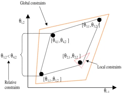
Local linear constraints applied to fuzzy models can be grouped into the follow- ing categories according to their validity region:

• Local constrains are valid only for the parameters of a regression model, Λ_iθ_i ≤ω_i.

• Global constrainsare related to all of the regression models,Λ_glθ_i ≤ω_gl, i= 1, . . . , c.

• Relative constrainsdefine the relative magnitude of the parameters of two or more regression models.

Λ_rel,i,j [ θ_i

θ_j ]

≤ω_rel,i,j (2.15)

An example for these types of constrains are illustrated in Fig.2.3.

In order to handle relative constraints, the set of weighted optimization problems has to be solved simultaneously. Hence, the constrained optimization problem is formulated as follows:

minθ

{1

2θ^THθ+c^Tθ }

(2.16)

θ

Global constraints

Local constraints [

θ

θ

θ

[

θ

θ

[

θ

θ

[

θ

θ

θ

θ

Relative constraints

Figure 2.3: Hinging hyperplane model with 4 local constraints and two parameters withH= 2X^′TΦX^′,c=−2X^′TΦy^′, where

y^′ =







 y y ... y









, θ =







 θ₁ θ₂ ... θ_c









, (2.17)

X^′ =









X1 0 · · · 0 0 X₂ · · · 0 ... ... . .. ... 0 0 · · · X_c









, Φ=









Φ1 0 · · · 0 0 Φ₂ · · · 0 ... ... . .. ...

0 0 · · · Φ_c









(2.18)

whereΦ_icontains local membership values and the constraints onθ:

Λθ≤ω (2.19)

with

Λ=























Λ₁ 0 · · · 0

0 Λ2 · · · 0

... ... . .. ...

0 0 · · · Λ_c

Λ_gl 0 · · · 0

0 Λ_gl · · · 0 ... ... . .. ...

0 0 · · · Λgl

{Λ_rel}





















 , ω =





















 ω₁ ω2

... ω_c ω_gl ω_gl ... ωgl

{ω_rel}























. (2.20)

Referring back to Fig.2.1 it can be concluded with this method both part of the intersected hyperplanes are described and that part (⟨max|min⟩) is selected which describes the the training data in the most accurate way.

2.2 Hinging hyperplane based binary trees

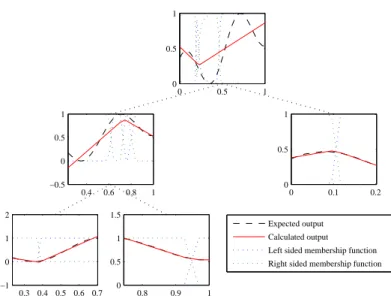
So far, the hinging hyperplane function identification method is presented. The pro- posed technique can be used to determine the parameters of one hinging hyperplane function. The classical hinging hyperplane approach can be interpreted by identi- fying K hinging hyperplane models consisting of global model pairs, since these operating regimes cover the wholeN dataset. This representation leads to several problems not just during model identification but also renders model interpretabil- ity more difficult. To overcome this problem a tree structure is proposed where the data is recursively partitioned into subsets, while each subset used to form models of lower levels of the tree. The concept is illustrated in Fig. 2.4, where the mem- bership functions and the identified hinging hyperplane models are also shown.

During the identification the following phenomena can be taken into consideration (that can be considered as benefits too):

• By using hinging hyperplane function there is no need to find splitting vari- ables at the nonterminal nodes, since this procedure is based on the hinge.

• Populated tree is always a binary tree either balanced, or non–balanced, de- pending on the algorithm (greedy or non–greedy). Based on binary tree, and the hinge splitting thexdata pertains to left side of the hingeθ₁always goes to the left child, and the right side behaves the same accordingly. For ex- ample given a simple symmetrical binary tree structure model, the first level

0 0.5 1 0

0.5 1

0.4 0.6 0.8 1

−0.5 0 0.5 1

0 0.1 0.2

0 0.5 1

0.3 0.4 0.5 0.6 0.7

−1 0 1 2

0.8 0.9 1

0 0.5 1 1.5

Expected output Calculated output Left sided membership function Right sided membership function

Figure 2.4: Hinging hyperplane based regression tree for basic data sample in case of greedy algorithm

contains one hinging hyperplane function, the second level contains 2 hinging hyperplane functions, the third level contains 4 hinges, and in general thekth level contains2^(k−1) hinging hyperplane functions.

Concluding the above and obtaining the parametersθ during recursive identifi- cation the following cost function has to be minimized:

E({θi}, π) =

∑K i=1

πiEmi(θi) (2.21)

whereKis the number of the hinge functions (nodes), andπis the binary (π_i ∈0,1) terminal set, indicating that the given node is a final linear model (π_i = 1), and can be incorporated as a terminal node of the identified piecewise model.

Growing algorithm can be either balanced or greedy. In balanced case the identifica- tion algorithm builds the tree till the desired stopping criteria, while the greedy one will continue the tree building with choosing a node for splitting which performs worst during the building procedure. Hence, this operating regime needs further local models for better model performance. For a greedy algorithm the crucial item is the selection of the good stopping criteria. Any of the followings can be used to determine whether to continue the tree growing process or stop the procedure:

1. The loss function becomes zero. This corresponds to the situation where the size of the data set is less or equal to the dimension of the hinge. Since the

hinging hyperplanes are located by linear least–squares. From least–squares theory, when the number of data is equal to the number of parameters to be determined, the result would be exact, given the matrix is not singular.

2. E =E1+E2, whereEi =∑_N

k=1µi,k

(yk−fi(xk;θi))2

represents the perfor- mances of the left and right hand side models of the hinge. During the growth of the binary tree, the loss function is always non-increasing, soE should be always smaller than the performance of the parent node. When no decrease is observed in loss function, when the tree growing should be stopped.

3. The tree building process reaches the pre-defined tree depth.

4. All of the identified terminal nodes performance meets an accuracy level (ε- error rate ). In this case it is not necessary to specify the depth of the tree, but it can cause overfitting of the model.

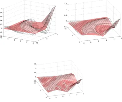
The algorithm results are represented in Fig. 2.4 where L = 3, K = 5, and π = [0,0,1,1,1]. On Fig. 2.5 a 3–dimensional example is shown. The function

y =

sin(√

x²₁+x²₂+ϵ )

√x²₁+x²₂+ϵ (2.22)

has been approximated by hinging hyperplane based tree. On Fig. 2.5 it is shown how the approximation becomes much more smoother with applying 1,2, and 4 level and greedy building method. Not just the generation of the binary tree structured model is important, but to construct a greedy algorithm and to measure the identified model, node performance must be determined during the identification procedure, which can be defined in different ways:

• Modeling performance of the nodes

The well–known regression performance estimators can be used for node performance measurement, in this work root mean squared prediction error (RMSE) was used.

RM SE = vu ut 1

N

∑N k=1

(yk−yˆk)² (2.23)

• Condition of the nodes