Fuzzy csoportosítás alkalmazása folyamatadatok elemzésében

DOKTORI (PhD) ÉRTEKEZÉS

FEIL BALÁZS

Pannon Egyetem

Pannon Egyetem Folyamatmérnöki Tanszék

Fuzzy csoportosítás alkalmazása folyamatadatok elemzésében

DOKTORI (PhD) ÉRTEKEZÉS

Feil Balázs

Konzulens

Dr. Abonyi János, egyetemi docens

Pannon Egyetem Vegyészmérnöki tudományok Doktori Iskolája

2006.

Fuzzy csoportosítás alkalmazása folyamatadatok elemzésében

Értekezés doktori (PhD) fokozat elnyerése érdekében a Pannon Egyetem Vegyészmérnöki tudományok

Doktori Iskolájához tartozóan.

Írta:

Feil Balázs

Konzulens: Dr. Abonyi János, egyetemi docens

Elfogadásra javaslom (igen / nem)

……….

(aláírás)

A jelölt a doktori szigorlaton…...% -ot ért el.

Az értekezést bírálóként elfogadásra javaslom:

Bíráló neve: …... …... igen /nem

……….

(aláírás)

Bíráló neve: …... …... igen /nem

……….

(aláírás)

A jelölt az értekezés nyilvános vitáján…...% -ot ért el.

Veszprém, ……….

a Bíráló Bizottság elnöke

A doktori (PhD) oklevél minősítése…...

………

Az EDT elnöke

K¨ osz¨ onetnyilv´ an´ıt´ as

Nem k¨onny˝u feladat k¨osz¨onetnyilv´an´ıt´ast ´ırni. K´enytelen vagyok visszan´ezni ´eletem egy lassan lez´ar´o- d´o szakasz´ara, ´es ´ert´ekelni azt. Sokan ´alltak mellettem ebben a h´arom ´evben, s˝ot nemcsak ´acsorogtak, hanem n´eha (vagy nem is annyira n´eha?) k´enytelenek voltak megt´amogatni, hogy folytatni tudjam azt, amit elkezdtem, ´es igyekeztem is befejezni. Sok mindenkit˝ol ´es sok mindent tanultam, nemcsak szakmailag.

Mindenekel˝ott szeretn´em megk¨osz¨onni a csal´adomnak, sz¨uleimnek, n˝ov´eremnek ´es b´aty´amnak a t¨urelm´et ´es azt a b´ator´ıt´o ´es biztos h´atteret, amelyet n´eha ´eszrev´etlen¨ul, gyakran nagyon is k´ezzelfog- hat´oan biztos´ıtottak sz´amomra. M´eg olyankor is b´ıztak bennem, amikor m´ar ´en sem. ´Es t¨obbnyire Nekik lett igazuk. Erre j´o bizony´ıt´ek, hogy most ´eppen ezeket a mondatokat fogalmazgatom. Szeretn´ek k¨osz¨onetet mondani az´ert is, mert gyakran nem kaptak bel˝olem t´ul sokat otthon, m´egis elviseltek, ´es nem k¨osz¨ontem meg el´eg sokszor azt, amit tettek ´ertem.

Szeretn´ek k¨osz¨onetet mondani t´emavezet˝omnek, dr. Abonyi J´anosnak az´ert a rengeteg id˝o´ert ´es energi´a´ert, amit r´am ´aldozott. Igyekeztem ezt megh´al´alni a munk´ammal, rem´elem, hogy siker¨ult is valamilyen szinten. K¨osz¨onet illeti dr. Szeifert Ferencet, mert tansz´ekvezet˝ok´ent bepillant´ast engedett tenni a tansz´ek ´elet´ebe, ´es ´ıgy egy val´odi k¨oz¨oss´eg tagj´anak ´erezhettem magam, valamint b´atran fordulhattam Hozz´a (is) szakmai probl´em´aimmal. K¨ul¨on ki kell emelnem a tansz´eki PhD hallgat´okat, Balask´o Bal´azst, dr. Mad´ar J´anost ´es Pach Ferenc P´etert, akikkel gyakran folytattunk legal´abbis sz´amomra inspir´al´o besz´elget´eseket - nemcsak szakmai t´em´akban.

K¨osz¨on¨om bar´ataimnak, illetve koll´egiumi szobat´arsaimnak azt, hogy t´arsas´agot ny´ujtottak vagy csak elviseltek, meghallgattak, amikor arra volt sz¨uks´eg. K¨ul¨on ki szeretn´em emelni k¨oz¨ul¨uk dr. Szele B´alintot, Tak´acs Levent´et, Borb´ely P´etert ´es Czig´any Attil´at, mert j´oform´an b´armikor fordulhattam Hozz´ajuk, ´es siker¨ult Nekik t´ag´ıtani a l´at´ok¨or¨omet, illetve a zenei ´ızl´esemet, valamint toleranci´at tanultam T˝ol¨uk magammal ´es m´asokkal szemben. K¨osz¨onet ´erte!

V´eg¨ul, de nem utols´o sorban szeretn´ek k¨osz¨onetet mondani mindazon egyetemi dolgoz´onak, aki

´atseg´ıtett az egyetemi adminisztr´aci´o ´utveszt˝oin, k¨ul¨on kiemelve B´eres Zsuzs´at ´es Bittmann G´aborn´et.

Feil Bal´azs

Veszpr´em, 2006 m´ajusa

Contents

1 Classical Fuzzy Cluster Analysis 5

1.1 Motivation . . . 5

1.2 Types of Data . . . 7

1.3 Similarity Measures . . . 8

1.4 Clustering Techniques . . . 10

1.4.1 Hierarchical Clustering Algorithms . . . 10

1.4.2 Partitional Algorithms . . . 12

1.5 Fuzzy Clustering . . . 15

1.5.1 Fuzzy partition . . . 15

1.5.2 The Fuzzy c-Means Functional . . . 16

1.5.3 Ways for Realizing Fuzzy Clustering . . . 16

1.5.4 The Fuzzy c-Means Algorithm . . . 17

1.5.5 Inner-Product Norms . . . 20

1.5.6 Gustafson–Kessel Algorithm . . . 21

1.5.7 Gath–Geva Clustering Algorithm . . . 23

1.6 Cluster Analysis of Correlated Data . . . 25

1.7 Validity Measures . . . 28

2 Clustering for Fuzzy Regression Tree Identification 30 2.1 Preliminaries . . . 34

2.2 Clustering based Identification . . . 36

2.2.1 Expectation-Maximization based Fuzzy Clustering for Regression Trees . . . . 36

2.2.2 Identification of Fuzzy Regression Trees . . . 39

2.2.3 Selection of the Splitting Variable . . . 41

2.2.4 Fine Tuning . . . 41

2.3 Conclusions . . . 45

3 Fuzzy Clustering for System Identification 46 3.1 Data-Driven Modeling of Dynamical Systems . . . 47

3.2 Model Order Selection . . . 51

3.2.1 Introduction . . . 51

3.2.2 FNN Algorithm . . . 53

3.2.3 Fuzzy Clustering based FNN . . . 54

3.2.4 Cluster Analysis based Direct Model Order Estimation . . . 56

3.2.5 Application Examples . . . 57

3.2.6 Conclusions . . . 63

3.3 State-Space Reconstruction . . . 64

3.3.1 Introduction . . . 64

3.3.2 Clustering-Based Approach to State Space Reconstruction . . . 65

3.3.3 Application Examples and Discussion . . . 72

3.3.4 Case Study . . . 79

3.3.5 Conclusions . . . 87

4 Segmentation of Multivariate Time-series 88 4.1 Mining Time-series Data . . . 88

4.2 Time-series Segmentation . . . 90

4.3 Fuzzy Cluster based Fuzzy Segmentation . . . 95

4.3.1 PCA based Distance Measure . . . 96

4.3.2 Clustering for Time-series Segmentation . . . 97

4.3.3 Automatic Determination of the Number of Segments . . . 98

4.3.4 Number of Principal Components . . . 101

4.3.5 The Segmentation Algorithm . . . 102

4.3.6 Case Studies . . . 102

4.4 Conclusions . . . 106

5 Kalman Filtering in Process Monitoring 107 5.1 Time Series Segmenation based on Kalman Filtering . . . 107

5.1.1 State-estimation based Segmentation . . . 108

5.1.2 Application example . . . 110

5.1.3 Conclusions . . . 116

5.2 Semi-mechanistic Models for State-estimation . . . 117

5.2.1 Problem description . . . 117

5.2.2 Semi-mechanistic model of the polimerization unit . . . 118

5.2.3 Spline-smoothing based identification of neural networks . . . 119

5.2.4 Conclusions . . . 121

6 Summary 122

Kivonat

Fuzzy csoportos´ıt´ as alkalmaz´ asa folyamatadatok elemz´ es´ eben

Napjaink technol´ogiai rendszereinek ¨uzemeltet´ese sor´an a v´altoz´ok, param´eterek sz´ama nagy ´es gyakran van sz¨uks´eg ezek ´ert´ekeire. Ez´ert a folyamatir´any´ıt´o rendszerek t¨obbs´ege rendelkezik az adatok r¨ogz´ıt´es´et biztos´ıt´o funkci´okkal. A lok´alis szint˝u (aktu´alis) feladatok megold´asa ut´an a v´altoz´ok ´es param´eterek ´ert´ekeinek ´un. ”id˝osora” marad, amelyet e rendszerekben k¨ul¨onb¨oz˝o m´odokon r¨ogz´ıtenek

´es archiv´alnak. A PhD dolgozat ´altal javasolt megold´asok kifejleszt´es´enek c´elja az volt, hogy lehet˝ov´e tegy¨uk, hogy a jellemz˝o v´altoz´ok id˝osoraiban nyilv´anval´oan benne l´ev˝o, de kor´abban fel nem ismert inform´aci´ok kinyerhet˝ok legyenek, az´ert, hogy a kinyert inform´aci´ok alkalmazhat´ov´a v´alljanak a tech- nol´ogia megismer´es´eben, ir´any´ıt´as´aban, optimaliz´al´as´aban ´es a tervez´esben. A megold´asok alapgon- dolata a k¨ovetkez˝o:

Az adatb´any´aszat egyik fontos ter¨ulete, az adatok csoportos´ıt´asa sokv´altoz´os adatok k¨oz¨otti ha- sonl´os´ag felt´ar´as´aval foglalkozik, azaz az adatok ´altal reprezent´alt objektumok olyan halmazait igyek- szik felkutatni, melyekbe tartoz´ok egym´ashoz hasonl´oak, m´ıg m´as halmazbeli elemekt˝ol k¨ul¨onb¨oznek.

A gyakorlatban gyakran nem lehet ´eles hat´arokat h´uzni a csoportok k¨oz´e, ez´ert az ´un. fuzzy halmazok elk¨ul¨on´ıt´ese (fuzzy csoportos´ıt´as) jobban visszat¨ukr¨ozi az emberi gondolkod´ast, mivel megengedi, hogy egy objektum t¨obb csoporthoz is tartozzon egyszerre. Olyan eszk¨oz¨oket dolgoztunk ki fuzzy csopor- tos´ıt´asi algoritmusok felhaszn´al´as´aval, melyek alkalmasak folyamatm´ern¨oki probl´em´ak megold´as´ara.

Fuzzy csoportos´ıt´asi algoritmusokat alkalmazunk, kombin´alunk egy´eb folyamatm´ern¨oki eszk¨oz¨okkel,

´ıgy ¨uzleti ´es technol´ogiai rendszerek ¨uzemel´es´enek nyomon k¨ovet´es´ere ´es diagn´ozis´ara, modellez´es´ere

´es identifik´aci´oj´ara alkalmas algoritmusok sz¨ulettek.

A sz´amtalan megold´as k¨oz¨ul a dolgozat csak n´eh´anyat ismertet. Hierarchikus fuzzy modellek (d¨ont´esi ´es regresszi´os f´ak) identifik´aci´oja, melyek kihaszn´alj´ak a d¨ont´esi f´ak kompakt tud´asreprezen- t´aci´oj´at, hogy kezelni tudj´ak a modellstrukt´ura meghat´aroz´as´at.

T¨obbv´altoz´os id˝osorok szegment´al´asa, ill. ´allapotbecsl˝o algoritmus felhaszn´al´asa a rendszer ´allapo- t´aban be´all´o v´altoz´asok k¨ovet´es´ere, ill. term´ekmin˝os´eg-becsl´esre. Ehhez val´osz´ın˝us´egi f˝okomponens- anal´ızis modellek (PPCA) kever´ek´en alapul´o m´odszert dolgoztunk ki, ´es a param´etereiknek ´es a szeg- mensek hat´arainak meghat´aroz´as´ara fuzzy csoportos´ıt´ason alapul´o eszk¨ozt fejlesztet¨unk. A kidolgo- zott eszk¨oz a f˝okomponensek ´es a szegmensek sz´am´anak automatikus meghat´aroz´as´ara is k´epes. Az algoritmus hat´ekonys´ag´at szintetikus ´es val´os, ipari adatsorok felhaszn´al´as´aval m´ar bizony´ıtottuk.

Allapotbecsl˝o algoritmus felhaszn´al´as´aval azonban a term´ekmin˝os´eg is becs¨´ ulhet˝o, amennyiben megfelel˝o modell ´all a rendelkez´es¨unkre. A vizsg´alt rendszer bonyolults´aga miatt azonban gyakran nincs elegend˝o a priori inform´aci´onk ezen feladat megold´as´ahoz. Ilyen esetekben ´erdemes a kev´esb´e ismert r´eszeket feketedoboz-modellekkel k¨ozel´ıteni ´es ezt a modellt be´ep´ıteni a rendszer feh´erdoboz- modellj´ebe. Az ilyen modelleket szemi-mechanisztikus modelleknek nevezz¨uk. Egy olyan modellez´esi keretrendszert dolgoztunk ki, melynek felhaszn´al´as´aval megoldhat´o a term´ek min˝os´eg´enek on-line becsl´ese.

Abstract

Fuzzy clustering in process data mining

Information about (chemical) processes to be modeled, controlled and optimized is limited and of various type because these (industrial) systems are so-called ’data rich-knowledge poor’ systems owing to their complexity. Tremendous measured data and operators’ experience are available, hence a new interdisciplinary science field, data mining, could shape with the aim of discovering knowledge based on data. Clustering is an important unsupervised technique of this new approach with the aim of partitioning the data sets into subsets containing similar samples (called clusters). The transitions between subsets can be crisp (hard partitioning) or gradual (fuzzy clustering). The thesis contributes to application of data mining methods in process engineering on the basis of technological data. The developed tools can be applied in many fields due to the generality of the problems and their solutions.

Auszug

Fuzzy Cluster-Analyse im Prozessdaten-bergbau

Informationen ¨uber die (chemischen) zu modellierenden Prozesse, verschiedener Weise gesteuert, op- timiert und kontrolliert, sind von ihrer Kompliziertheit begrenzt, weil diese (industriellen) Systeme sind sogenannte ’Reich an Daten - arm an Kentnisse’ Systeme. Enorme gemessene Daten- und Oper- atorerfahrung sind vorhanden, dadurch konnte eine neue interdisziplin¨are Wissenschaft aufgefangen,

’Daten-Bergbau’, mit dem Ziel des Entdeckens des Wissens zu formen. Das Cluster-Analyse ist eine un¨uberwachte Technik dieser neuen Ann¨aherung mit dem Ziel des Einteilens den Daten in ¨ahnlichen Partien (genannt Clusters). Diese ¨Uberg¨ange zwischen Partien k¨onnen scharf (hartes Einteilen) oder stufenweise (Fuzzy Clustering) sein. Die These tr¨agt zur Anwendung der Datengewinnenmethoden in der Prozesstechnik auf der Grundlage von technologische Daten bei. Die entwickelten Werkzeuge k¨onnen wegen des Allgemeinen der Probleme und ihrer L¨osungen in vielen wissenschaftlichen Sparten angewendet werden.

Preface

Overview

In the last decade the amount of the stored data has rapidly increased related to almost all areas of life. The most recent survey was given by Berkeley University of California about the amount of data. According to that, data occurred only in 2002 and stored in pressed media, films and electronics devices are about 5 exabytes. For comparing purposes, if all the 19 million volumes of Library of Congress of the United States of America were digitalized, it would be only 10 terabytes. Hence, 5 exabytes is about a half million Library of Congress. If this data mass is projected into 6.3 billion inhabitants of Earth, then it roughly means that each contemporary generates 800 megabytes of data every year. It is interesting to compare this amount with Shakespeare’s life-work, which can be stored even in 5 megabytes. The reason is that the tools that make it possible have been developing in an impressive way, consider e.g. the development of measuring tools and data collectors in production units, and their support information systems. This progress has been induced by the fact that systems are often been used in engineering or financial-business practice that we do not know in depth and we need more information about them. This lack of knowledge should be compensated by the mass of the stored data that is available nowadays. It can also be the case that the causality is reversed:

the available data have induced the need to process and use them, e.g. web mining. The data reflect the behavior of the analyzed system, therefore there is at least the theoretical potential to obtain useful information and knowledge from data. On the ground of that need and potential a distinct science field grew up using many tools and results of other science fields: data mining or more general, knowledge discovery in databases.

Historically the notion of finding useful patterns in data has been given a variety of names including data mining, knowledge extraction, information discovery, and data pattern processing. The term data mining has been mostly used by statisticians, data analysts, and the management information systems communities.

The term knowledge discovery in databases (KDD) refers to the overall process of discovering knowledge from data, while data mining refers to a particular step of this process. Data mining is the application of specific algorithms for extracting patterns from data. The additional steps in the KDD process, such as data selection, data cleaning, incorporating appropriate prior knowledge, and proper interpretation of the results are essential to ensure that useful knowledge is derived form the data.

KDD has evolved from the intersection of research fields such as machine learning, pattern recog- nition, databases, statistics, artificial intelligence, and more recently it gets new inspiration from computational intelligence.

Brachman and Anand give a practical view of the KDD process emphasizing the interactive nature of the process. Here we broadly outline some of its basic steps depicted in Figure 1, and we show the connections of these steps to CI based models and algorithms.

1. Developing and understanding of the application domain and the relevant prior knowledge, and identifying the goal of the KDD process. The transparency of fuzzy systems allows the user to

Figure 1: Steps of the knowledge discovery process.

effectively combine different types of information, namely linguistic knowledge, first-principle knowledge and information from data.

2. Creating target data set.

3. Data cleaning and preprocessing: basic operations such as the removal of noise, handling missing data fields.

4. Data reduction and projection: finding useful features to represent the data depending the goal of the task. Using dimensionality reduction or transformation methods to reduce the effective number of variables under consideration or to find invariant representation of data. Neural networks, cluster analysis, and neuro-fuzzy systems are often used for this purpose.

5. Matching the goals of the KDD process to a particulardata mining method: Although the boundaries between prediction and description are not sharp, the distinction is useful for un- derstanding the overall discovery goal. The goals of data mining are achieved via the following data mining methods:

• Clustering: Identification a finite set of categories or clusters to describe the data. Closely related to clustering is the method of probability density estimation. Clustering quantizes the available input-output data to get a set of prototypes and use the obtained prototypes (signatures, templates, etc., and many writers refer to as codebook) and use the prototypes as model parameters.

• Summation: finding a compact description for subset of data, e.g. the derivation of summary for association of rules and the use of multivariate visualization techniques.

• Dependency modeling: finding a model which describes significant dependencies be- tween variables (e.g. learning of belief networks).

• Regression: learning a function which maps a data item to a real-valued prediction vari- able and the discovery of functional relationships between variables.

• Classification: learning a function that maps (classifies) a data item into one of several predefined classes.

• Change and Deviation Detection: Discovering the most significant changes in the data from previously measured or normative values.

6. Choosing thedata mining algorithm(s): selecting algorithms for searching for patterns in the data. This includes deciding which model and parameters may be appropriate and matching a particular algorithm with the overall criteria of the KDD process (e.g. the end-user may be more interested in understanding the model than its predictive capabilities.) One can identify three

primary components in any data mining algorithm: model representation, model evaluation, and search.

• Model representation: the language is used to describe the discoverable patterns. If the representation is too limited, then no amount of training time or examples will produce an accurate model for the data. Note that more powerful representation of models increases the danger of overfitting the training data resulting in reduced prediction accuracy on unseen data. It is important that a data analysts fully comprehend the representational assumptions which may be inherent in a particular method.

For instance, rule-based expert systems are often applied to classification problems in fault detection, biology, medicine etc. Among the wide range of CI techniques, fuzzy logic improves classification and decision support systems by allowing the use of overlapping class definitions and improves the interpretability of the results by providing more insight into the classifier structure and decision making process.

• Model evaluation criteria: qualitative statements or fit functions of how well a particu- lar pattern (a model and its parameters) meet the goals of the KDD process. For example, predictive models can often be judged by the empirical prediction accuracy on some test set. Descriptive models can be evaluated along the dimensions of predictive accuracy, nov- elty, utility, and understandability of the fitted model. Traditionally, algorithms to obtain classifiers have focused either on accuracy or interpretability. Recently some approaches to combining these properties have been reported

• Search method: consists of two components: parameter search and model search. Once the model representation and the model evaluation criteria are fixed, then the data mining problem has been reduced to purely an optimization task: find the parameters/models for the selected family which optimize the evaluation criteria given observed data and fixed model representation. Model search occurs as a loop over the parameter search method.

The automatic determination of fuzzy classification rules from data has been approached by several different techniques: neuro-fuzzy methods, genetic-algorithm based rule selection and fuzzy clustering in combination with GA-optimization. For high-dimensional classifi- cation problems, the initialization step of the identification procedure of the fuzzy model becomes very significant.

7. Data mining: searching for patterns of interest in a particular representation form or a set of such representations: classification rules or trees, regression. Some of the CI models lend themselves to transform into other model structure that allows information transfer between different models (e.g. a decision tree mapped into a feedforward neural network or radial basis functions are functionally equivalent to fuzzy inference systems).

8. Interpreting mined patterns, possibly return to any of steps 1-7 for further iteration. This step can also involve the visualization of the extracted patterns/models, or visualization of the data given the extracted models.

9. Consolidating discovered knowledge: incorporating this knowledge into another system for fur- ther action, or simply documenting and reporting it.

When we attempt to solve realworld problems, like extracting knowledge from large amount of data, we realize that they are typically illdefined systems, difficult to model and with largescale solu- tion spaces. In these cases, precise models are impractical, too expensive, or nonexistent. Furthermore, the relevant available information is usually in the form of empirical prior knowledge and input-output data representing instances of the system’s behavior. Therefore, we need an approximate reasoning

systems capable of handling such imperfect information. Computational Intelligence (CI) and Soft Computing (SC) are recently coined terms describing the use of many emerging computing disciplines.

According to Zadeh (1994): ”... in contrast to traditional, hard computing, soft computing is tolerant of imprecision, uncertainty, and partial truth.” In this context Fuzzy Logic (FL), Probabilistic Reason- ing (PR), Neural Networks (NNs), and Genetic Algorithms (GAs) are considered as main components of CI. Each of these technologies provide us with complementaryreasoningandsearchingmethods to solve complex, realworld problems. What is important to note is that soft computing is not a melange. Rather, it is a partnership in which each of the partners contributes a distinct methodology for addressing problems in its domain. In this perspective, the principal constituent methodologies in CI are complementary rather than competitive.

Because of the different data sources and user needs the purpose of data mining methods may be varied in a range field. The new results presented in this thesis cover a range of topic, but they are similar in the applied method: fuzzy clustering algorithms were used for all of them. One important field within data mining is clustering that deals with discovering similarity among (multivariate) data.

Hence, it tries to discover and separate sets in which data are more similar to each other since data from different sets are less similar. In practice it is often the case that crisp borders between clusters cannot be determined, that is why so-called fuzzy clustering is much closer to the human thinking since it allows one point to belong to more clusters simultaneously. Clustering algorithms can be applied in many areas and for many purposes. The objective of the present thesis work was to develop methods using fuzzy clustering algorithms that are able to solve process engineering problems. According to that, this thesis deals with the following:

• fuzzy model identification emphasized the interpretability and transparency or the results (Chap- ter 2);

• model order selection of input-output as well as autonomous systems (Chapter 3);

• segmentation of multivariate time-series (Chapter 4);

• and application of state estimation algorithm to detect changes in the state of the system and for product quality estimation (Chapter 5).

Chapter 1

Classical Fuzzy Cluster Analysis

1.1 Motivation

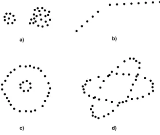
The goal of clustering is to determine the intrinsic grouping in a set of unlabeled data. Data can reveal clusters of different geometrical shapes, sizes and densities as demonstrated in Figure 1.1. Clusters can be spherical (a), elongated or ”linear” (b), and also hollow (c) and (d). Their prototypes can be points (a), lines (b), spheres (c) or ellipses (d) or their higher dimensional analogs. Clusters (b) to (d) can be characterized as linear and nonlinear subspaces of the data space (R² in this case).

Algorithms that can detect subspaces of the data space are of particular interest for identification.

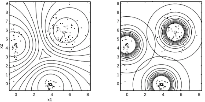
The performance of most clustering algorithms is influenced not only by the geometrical shapes and densities of the individual clusters but also by the spatial relations and distances among the clusters.

Clusters can be well-separated, continuously connected to each other, or overlapping each other. The separation of clusters is influenced by the scaling and normalization of the data (see Example 1.1, Example 1.2 and Example 1.3).

Figure 1.1: Clusters of different shapes inR².

The goal of this section is to survey the core concepts and techniques in the large subset of cluster analysis, and to give detailed description about the fuzzy clustering methods applied in the remainder chapters of this thesis.

Typical pattern clustering activity involves the following steps [85]:

1. Pattern representation (optionally including feature extraction and/or selection).

Pattern representation refers to the number of classes, the number of available patterns, and the number, type, and scale of the features available to the clustering algorithm. Some of this information may not be controllable by the practitioner. Feature selection is the process of identifying the most effective subset of the original features to use in clustering. Feature extraction is the use of one or more transformations of the input features to produce new salient features. Either or both of these techniques can be used to obtain an appropriate set of features to use in clustering.

2. Definition of a pattern proximity measure appropriate to the data domain.

Pattern proximity is usually measured by a distance function defined on pairs of patterns. A variety of distance measures are in use in the various communities [12, 46, 85]. A simple distance measure like Euclidean distance can often be used to reflect dissimilarity between two patterns, whereas other similarity measures can be used to characterize the conceptual similarity between patterns [126] (see Section 1.3 for more details).

3. Clustering or grouping.

The grouping step can be performed in a number of ways. The output clustering (or clusterings) can be hard (a partition of the data into groups) or fuzzy (where each pattern has a variable degree of membership in each of the clusters). Hierarchical clustering algorithms produce a nested series of partitions based on a criterion for merging or splitting clusters based on simi- larity. Partitional clustering algorithms identify the partition that optimizes (usually locally) a clustering criterion. Additional techniques for the grouping operation include probabilistic [32]

and graph-theoretic [180] clustering methods (see also Section 1.4).

4. Data abstraction (if needed).

Data abstraction is the process of extracting a simple and compact representation of a data set. Here, simplicity is either from the perspective of automatic analysis (so that a machine can perform further processing efficiently) or it is human-oriented (so that the representation obtained is easy to comprehend and intuitively appealing). In the clustering context, a typical data abstraction is a compact description of each cluster, usually in terms of cluster prototypes or representative patterns such as the centroid [46]. A low dimensional graphical representation of the clusters could also be very informative, because one can cluster by eye and qualitatively validate conclusions drawn from clustering algorithms (see e.g. Kohonen Self-Organizing Maps [103], auto-associative feed-forward networks [105], Sammon mapping [121, 140] and fuzzy Sam- mon mapping [104]).

5. Assessment of output (if needed).

How is the output of a clustering algorithm evaluated? What characterizes a good clustering result and a poor one? All clustering algorithms will, when presented with data, produce clusters regardless of whether the data contain clusters or not. If the data does contain clusters, some clustering algorithms may obtain better clusters than others. The assessment of a clustering procedures output, then, has several facets. One is actually an assessment of the data domain rather than the clustering algorithm itself data which do not contain clusters should not be processed by a clustering algorithm. The study of cluster tendency, wherein the input data are examined to see if there is any merit to a cluster analysis prior to one being performed, is a relatively inactive research area. The interested reader is referred to [42] and [51] for more information.

The goal of clustering is to determine the intrinsic grouping in a set of unlabeled data. But how to decide what constitutes a good clustering? It can be shown that there is no absolute ’best’ criterion which would be independent of the final aim of the clustering. Consequently, it is the user which must supply this criterion, in such a way that the result of the clustering will suit their needs. In spite of that, a ’good’ clustering algorithm must give acceptable results in many kinds of problems besides other requirements. In practice, the accuracy of a clustering algorithm is usually tested on well-known labeled data sets. It means that classes are known in the analyzed data set but certainly they are not used in the clustering. Hence, there is a benchmark to qualify the clustering method, and the accuracy can be represented by numbers (e.g. percentage of misclassified data).

Cluster validity analysis, by contrast, is the assessment of a clustering procedures output.

Often this analysis uses a specific criterion of optimality; however, these criteria are usually arrived at subjectively. Hence, little in the way of gold standards exist in clustering except in well-prescribed subdomains. Validity assessments are objective [52] and are performed to determine whether the output is meaningful. A clustering structure is valid if it cannot reasonably have occurred by chance or as an artifact of a clustering algorithm. When statistical approaches to clustering are used, validation is accomplished by carefully applying statistical methods and testing hypotheses. There are three types of validation studies. An external assessment of validity compares the recovered structure to an a priori structure. An internal examination of validity tries to determine if the structure is intrinsically appropriate for the data. A relative test compares two structures and measures their relative merit.

Indices used for this comparison are discussed in detail in [52] and [85], and in Section 1.7.

1.2 Types of Data

The expression ’data’ has been mentioned several times in the previous short paragraph. Being loyal to the traditional scientific conventionality, this expression needs to be explained.

Data can be ’relative’ or ’absolute’. ’Relative data’ means that their values are not, but their pairwise distance are known. These distances can be arranged as a matrix called proximity matrix.

It can also be viewed as a weighted graph. See also Section 1.4.1 where hierarchical clustering is described that uses this proximity matrix. In this thesis mainly’absolute data’ is considered, so some more accurate expressions should be given about this.

The types of absolute data can be arranged in four categories. Letxand x⁰ be two values of the same attribute.

1. Nominal type. In this type of data, the only thing that can be said about two data if they are the same or not: x=x⁰ orx6=x⁰.

2. Ordinal type. The values can be arranged in a sequence. Ifx6=x⁰, then it is also decidable that x > x⁰ orx < x⁰.

3. Interval scale. If the difference between two data items can be expressed as a number besides the above-mentioned terms.

4. Ratio scale. This type of data is interval scale but zero value exists as well. Ifc = _x^x0, then it can be said thatxisc times biggerx⁰.

In this thesis, the clustering of ratio scale data is considered. The data are typically observations of some physical processes. In these cases, not only one butnvariables are measured simultaneously, therefore each observation consists of n measured variables, grouped into an n-dimensional column vector x_k = [x_1,k, x_2,k, . . . , x_n,k]^T, x_k ∈Rⁿ. These variables are usually not independent from each

other, therefore multivariate data analysis is needed that is able to handle these observations. A set ofN observations is denoted byX={xk|k= 1,2, . . . , N}, and is represented as anN×nmatrix:

X=







x1,1 x1,2 · · · x1,n

x2,1 x2,2 · · · x2,n

... ... . .. ... xN,1 xN,2 · · · xN,n





. (1.1)

In pattern recognition terminology, the rows of X are called patterns or objects, the columns are called thefeaturesor attributes, andXis called thepattern matrix. In this thesis,Xis often referred to simply as the data matrix. The meaning of the rows and columns of X with respect to reality depends on the context. In medical diagnosis, for instance, the rows of X may represent patients, and the columns are then symptoms, or laboratory measurements for the patients. When clustering is applied to the modeling and identification of dynamic systems, the rows of Xcontain samples of time signals, and the columns are, for instance, physical variables observed in the system (position, velocity, temperature, etc.).

In system identification, the purpose of clustering is to find relationships between independent system variables, called the regressors, and future values of dependent variables, called the regressands.

One should, however, realize that the relations revealed by clustering are just acausal associations among the data vectors, and as such do not yet constitute a prediction model of the given system. To obtain such a model, additional steps are needed which will be presented in Section 3.2. In order to represent the system’s dynamics, past values of the variables are typically included inXas well.

Data can be given in the form of a so-called dissimilarity matrix:







0 d(1,2) d(1,3) · · · d(1, N) 0 d(2,3) · · · d(2, N)

0 . .. ... 0





 (1.2)

whered(i, j) means the measure of dissimilarity (distance) between objectxiandxj. Becaused(i, i) = 0,∀i, zeros can be found in the main diagonal, and that matrix is symmetric becaused(i, j) =d(j, i).

There are clustering algorithms that use that form of data (e.g. hierarchical methods). If data are given in the form of (1.1), the first step that has to be done is to transform data into dissimilarity matrix form.

1.3 Similarity Measures

Dealing with clustering methods like in this thesis, ’What are clusters?’ can be the most important question. Various definitions of a cluster can be formulated, depending on the objective of clustering.

Generally, one may accept the view that a cluster is a group of objects that are more similar to one another than to members of other clusters. It is important to emphasize that more specific definition of clusters can hardly be formulated because the various type of problems and aims. Besides this problem, another crucial one is the enormous search space. IfN data points should be grouped byk clusters, the number of the possible (hard) clusterings is given by the Stirling numbers as follows:

S_N^(k)= 1 k!

Xk i=0

(−1)^k−i µk

i

¶

i^N. (1.3)

Even if there is only a small data set to be clustered, the possible number of clusterings is incredibly large. E.g., 25 data points into 5 clusters can be partitioned inS₂₅⁽⁵⁾= 2,436,684,974,110,751 different

ways. In addition, if the number of clusters are not known, the search space is even larger (P₂₅

k=1S₂₅^(k)>

4·10¹⁸). However, there is a need to cluster the data automatically, and objective definition should be formulated for the similarity and the quality of the clustering, because if the clustering is embedded by a mathematical model, there is the possibility to solve these problems quickly and effectively.

The term ”similarity” should be understood as mathematical similarity, measured in some well- defined sense. In metric spaces, similarity is often defined by means of a distance norm. Distance can be measured among the data vectors themselves, or as a distance form a data vector to some prototypical object of the cluster. The prototypes are usually not known beforehand, and are sought by the clustering algorithms simultaneously with the partitioning of the data. The prototypes may be vectors of the same dimension as the data objects, but they can also be defined as ”higher-level”

geometrical objects, such as linear or nonlinear subspaces or functions.

Since similarity is fundamental to the definition of a cluster, a measure of the similarity between two patterns drawn from the same feature space is essential to most clustering procedures. Because of the variety of feature types and scales, the distance measure (or measures) must be chosen carefully. It is most common to calculate the dissimilarity between two patterns using a distance measure defined on the feature space. We will focus on the well-known distance measures used for patterns whose features are all continuous.

The most popular metric for continuous features is theEuclidean distance

d2(xi,xj) = Ã _d

X

k=1

(xi,k−xj,k)²

!1/2

=kxi−xjk2, (1.4)

which is a special case (p= 2) of theMinkowski metric

dp(xi,xj) = Ã _d

X

k=1

|xi,k−xj,k|^p

!1/p

=kxi−xjkp. (1.5)

The Euclidean distance has an intuitive appeal as it is commonly used to evaluate the proximity of objects in two or three-dimensional space. It works well when a data set has compact or ”isolated”

clusters [120]. The drawback to direct use of the Minkowski metrics is the tendency of the largest-scaled feature to dominate the others. Solutions to this problem include normalization of the continuous features (to a common range or variance) or other weighting schemes. Linear correlation among features can also distort distance measures; this distortion can be alleviated by applying a whitening transformation to the data or by using the squaredMahalanobis distance

dM(xi,xj) = (xi−xj)F⁻¹(xi−xj)^T (1.6) where the patternsxi andxj are assumed to be row vectors, andFis the sample covariance matrix of the patterns or the known covariance matrix of the pattern generation process;dM(·,·) assigns different weights to different features based on their variances and pairwise linear correlations. Here, it is implicitly assumed that class conditional densities are unimodal and characterized by multidimensional spread, i.e., that the densities are multivariate Gaussian. The regularized Mahalanobis distance was used in [120] to extract hyperellipsoidal clusters. Recently, several researchers [53, 83] have used the Hausdorff distance in a point set matching context. Some clustering algorithms work on a matrix of proximity values instead of on the original pattern set. It is useful in such situations to precompute all theN(N−1)/2 pairwise distance values for theN patterns and store them in a (symmetric) matrix (see Section 1.2).

So far, only continuous variables have been dealt with. There are a lot of similarity measures for binary variables (see e.g. in [75]), but only continuous variables are considered in this thesis.

1.4 Clustering Techniques

Different approaches to clustering data can be described with the help of the hierarchy shown in Figure 1.2 (other taxonometric representations of clustering methodology are possible; ours is based on the discussion in [85]). At the top level, there is a distinction between hierarchical and partitional approaches (hierarchical methods produce a nested series of partitions, while partitional methods produce only one).

Clustering

Hierarchical Partitional

Single link Complete link Square error Graph theoretic

Mixture resolving

Mode seeking Figure 1.2: A taxonomy of clustering approaches.

1.4.1 Hierarchical Clustering Algorithms

A hierarchical algorithm yields a dendrogram representing the nested grouping of patterns and sim- ilarity levels at which groupings change. The dendrogram can be broken at different levels to yield different clusterings of the data. An example can be seen of Figure 1.3. On the left side, the interpat- tern distances can be seen in a form of dissimilarity matrix (1.2). In this initial state every point forms a single cluster. Thefirst step is to find the most similar two clusters (the nearest two data points).

In this example, there are two pairs with the same distance, choose one of them arbitrarily (B and E here). Write down the signs of the points, and connect them according to the figure, where the length of the vertical line is equal to the half of the distance. In thesecond step the dissimilarity matrix should be refreshed because the connected points form a single cluster, and the distances between this new cluster and the former ones should be computed. These steps should be iterated until only one cluster remains or the predetermined number of clusters is reached.

Most hierarchical clustering algorithms are variants of the single-link [159], complete-link [99], and minimum-variance [90, 130] algorithms. Of these, the single-link and complete-link algorithms are most popular. These two algorithms differ in the way they characterize the similarity between a pair of clusters. In the single-link method, the distance between two clusters is the minimum of the distances between all pairs of patterns drawn from the two clusters (one pattern from the first cluster, the other from the second). In the complete-link algorithm, the distance between two clusters is the maximum of all pairwise distances between patterns in the two clusters. In either case, two clusters are merged to form a larger cluster based on minimum distance criteria. The complete-link algorithm produces tightly bound or compact clusters [21]. The single-link algorithm, by contrast, suffers from a chaining effect [131]. It has a tendency to produce clusters that are straggly or elongated. The clusters obtained by the complete-link algorithm are more compact than those obtained by the single- link algorithm. The single-link algorithm is more versatile than the complete-link algorithm, otherwise.

However, from a pragmatic viewpoint, it has been observed that the complete-link algorithm produces more useful hierarchies in many applications than the single-link algorithm [85].

Figure 1.3: Dendrogram building [75].

0 0.5 1 1.5 2 2.5 3 3.5

0 0.5 1 1.5 2 2.5 3 3.5

1 151013 2 9 3 12 7 18 5 1920 6 14 4 1116 8 172131282225373827303924293235263436402333 0

0.2 0.4 0.6 0.8 1 1.2 1.4 1.6 1.8

Level

Figure 1.4: Partitional and hierarchical clustering results.

A simple example can be seen in Figure 1.4. On the left side, the blue dots depict the original data.

It can be seen that there are two well-separated clusters. The results of the single-linkage algorithm can be found on the right side. It can be determined that distances between data in the right cluster are greater than in the left one, but the two clusters can be separated well.

1.4.2 Partitional Algorithms

A partitional clustering algorithm obtains a single partition of the data instead of a clustering struc- ture, such as the dendrogram produced by a hierarchical technique. The difference of the two men- tioned methods can be seen in Figure 1.4. Partitional methods have advantages in applications involving large data sets for which the construction of a dendrogram is computationally prohibitive.

Squared Error Algorithms

The most intuitive and frequently used criterion function in partitional clustering techniques is the squared error criterion, which tends to work well with isolated and compact clusters. The squared error for a clusteringV={vi|i= 1, . . . , c} of a pattern setX(containingc clusters) is

J(X;V) = Xc i=1

X

k∈i

kx⁽ⁱ⁾_k −vik², (1.7)

wherex⁽ⁱ⁾_k is thekth pattern belonging to theith cluster andviis the centroid of theith cluster (see Algorithm 1.4.1).

Algorithm 1.4.1 (Squared Error Clustering Method).

1. Select an initial partition of the patterns with a fixed number of clusters and cluster centers.

2. Assign each pattern to its closest cluster center and compute the new cluster centers as the centroids of the clusters. Repeat this step until convergence is achieved, i.e., until the cluster membership is stable.

3. Merge and split clusters based on some heuristic information, optionally repeating step 2.

The k-means is the simplest and most commonly used algorithm employing a squared error criterion [124]. It starts with a random initial partition and keeps reassigning the patterns to clusters based on the similarity between the pattern and the cluster centers until a convergence criterion is met (e.g., there is no reassignment of any pattern from one cluster to another, or the squared error ceases to decrease significantly after some number of iterations). The k-means algorithm is popular because it is easy to implement, and its time complexity is O(N), where N is the number of patterns. A major problem with this algorithm is that it is sensitive to the selection of the initial partition and may converge to a local minimum of the criterion function value if the initial partition is not properly chosen. The whole procedure can be found in Algorithm 1.4.2.

Algorithm 1.4.2 (k-Means Clustering).

1. Choose k cluster centers to coincide with k randomly-chosen patterns or k randomly defined points inside the hypervolume containing the pattern set.

2. Assign each pattern to the closest cluster center.

3. Recompute the cluster centers using the current cluster memberships.

4. If a convergence criterion is not met, go to step 2. Typical convergence criteria are: no (or minimal) reassignment of patterns to new cluster centers, or minimal decrease in squared error.

Several variants of the k-means algorithm have been reported in the literature [12]. Some of them attempt to select a good initial partition so that the algorithm is more likely to find the global minimum value.

A problem accompanying the use of a partitional algorithm is the choice of the number of desired output clusters. A seminal paper [51] provides guidance on this key design decision. The partitional techniques usually produce clusters by optimizing a criterion function defined either locally (on a subset of the patterns) or globally (defined over all of the patterns). Combinatorial search of the set of possible labelings for an optimum value of a criterion is clearly computationally prohibitive. In practice, therefore, the algorithm is typically run multiple times with different starting states, and the best configuration obtained from all of the runs is used as the output clustering.

Another variation is to permit splitting and merging of the resulting clusters. Typically, a cluster is split when its variance is above a pre-specified threshold, and two clusters are merged when the distance between their centroids is below another pre-specified threshold. Using this variant, it is possible to obtain the optimal partition starting from any arbitrary initial partition, provided proper threshold values are specified. The well-known ISODATA algorithm employs this technique of merging and splitting clusters [23].

Another variation of the k-means algorithm involves selecting a different criterion function alto- gether. The dynamic clustering algorithm (which permits representations other than the centroid for each cluster) was proposed in [46, 163] and describes a dynamic clustering approach obtained by for- mulating the clustering problem in the framework of maximum-likelihood estimation. The regularized Mahalanobis distance was used in [120] to obtain hyperellipsoidal clusters.

The taxonomy shown in Figure 1.2 must be supplemented by a discussion of cross-cutting issues that may (in principle) affect all of the different approaches regardless of their placement in the taxonomy.

• Hard vs. fuzzy. A hard clustering algorithm allocates each pattern to a single cluster during its operation and in its output. A fuzzy clustering method assigns degrees of membership in several clusters to each input pattern. A fuzzy clustering can be converted to a hard clustering by assigning each pattern to the cluster with the largest measure of membership.

• Agglomerative vs. divisive. This aspect relates to algorithmic structure and operation (mostly in hierarchical clustering, see Section 1.4.1). An agglomerative approach begins with each pat- tern in a distinct (singleton) cluster, and successively merges clusters together until a stopping criterion is satisfied. A divisive method begins with all patterns in a single cluster and performs splitting until a stopping criterion is met.

• Monothetic vs. polythetic. This aspect relates to the sequential or simultaneous use of features in the clustering process. Most algorithms are polythetic; that is, all features enter into the

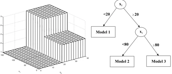
computation of distances between patterns, and decisions are based on those distances. A simple monothetic algorithm reported in [12] considers features sequentially to divide the given collection of patterns. The major problem with this algorithm is that it generates 2n clusters where n is the dimensionality of the patterns. For large values of n (n > 100 is typical in information retrieval applications [152]), the number of clusters generated by this algorithm is so large that the data set is divided into uninterestingly small and fragmented clusters.

• Deterministic vs. stochastic. This issue is most relevant to partitional approaches designed to optimize a squared error function. This optimization can be accomplished using traditional techniques or through a random search of the state space consisting of all possible labelings.

• Incremental vs. non-incremental. This issue arises when the pattern set to be clustered is large, and constraints on execution time or memory space affect the architecture of the algorithm. The early history of clustering methodology does not contain many examples of clustering algorithms designed to work with large data sets, but the advent of data mining has fostered the development of clustering algorithms that minimize the number of scans through the pattern set, reduce the number of patterns examined during execution, or reduce the size of data structures used in the algorithms operations.

A cogent observation in [85] is that the specification of an algorithm for clustering usually leaves considerable flexibility in implementation. In the following, we briefly discuss other clustering tech- niques as well, but a separate section (Section 1.5) and deep description are devoted to fuzzy clustering methods which are the most important in this thesis. Note that methods described in the next chapters are based on mixture of models as it is described in the following as well.

Mixture-Resolving and Mode-Seeking Algorithms

The mixture resolving approach to cluster analysis has been addressed in a number of ways. The un- derlying assumption is that the patterns to be clustered are drawn from one of several distributions, and the goal is to identify the parameters of each and (perhaps) their number. Most of the work in this area has assumed that the individual components of the mixture density are Gaussian, and in this case the parameters of the individual Gaussians are to be estimated by the procedure. Tradi- tional approaches to this problem involve obtaining (iteratively) a maximum likelihood estimate of the parameter vectors of the component densities [85]. More recently, the Expectation Maximization (EM) algorithm (a general purpose maximum likelihood algorithm [45] for missing-data problems) has been applied to the problem of parameter estimation. A recent thesis [127] provides an accessible description of the technique. In the EM framework, the parameters of the component densities are unknown, as are the mixing parameters, and these are estimated from the patterns. The EM pro- cedure begins with an initial estimate of the parameter vector and iteratively rescores the patterns against the mixture density produced by the parameter vector. The rescored patterns are then used to update the parameter estimates. In a clustering context, the scores of the patterns (which essen- tially measure their likelihood of being drawn from particular components of the mixture) can be viewed as hints at the class of the pattern. Those patterns, placed (by their scores) in a particular component, would therefore be viewed as belonging to the same cluster. Nonparametric techniques for density-based clustering have also been developed [85]. Inspired by the Parzen window approach to nonparametric density estimation, the corresponding clustering procedure searches for bins with large counts in a multidimensional histogram of the input pattern set. Other approaches include the application of another partitional or hierarchical clustering algorithm using a distance measure based on a nonparametric density estimate.

Nearest Neighbor Clustering

Since proximity plays a key role in our intuitive notion of a cluster, nearest neighbor distances can serve as the basis of clustering procedures. An iterative procedure was proposed in [118]; it assigns each unlabeled pattern to the cluster of its nearest labeled neighbor pattern, provided the distance to that labeled neighbor is below a threshold. The process continues until all patterns are labeled or no additional labelings occur. The mutual neighborhood value (described earlier in the context of distance computation) can also be used to grow clusters from near neighbors.

Graph-Theoretic Clustering.

The best-known graph-theoretic divisive clustering algorithm is based on construction of the minimal spanning tree (MST) of the data [180], and then deleting the MST edges with the largest lengths to generate clusters.

The hierarchical approaches are also related to graph-theoretic clustering. Single-link clusters are subgraphs of the minimum spanning tree of the data [68] which are also the connected components [67]. Complete-link clusters are maximal complete subgraphs, and are related to the node colorability of graphs [20]. The maximal complete subgraph was considered the strictest definition of a cluster in [15, 149]. A graph-oriented approach for non-hierarchical structures and overlapping clusters is presented in [138]. The Delaunay graph (DG) is obtained by connecting all the pairs of points that are Voronoi neighbors. The DG contains all the neighborhood information contained in the MST and the relative neighborhood graph (RNG) [168].

1.5 Fuzzy Clustering

Since clusters can formally be seen as subsets of the data set, one possible classification of clustering methods can be according to whether the subsets are fuzzy or crisp (hard). Hard clustering methods are based on classical set theory, and require that an object either does or does not belong to a cluster.

Hard clustering in a data set X means partitioning the data into a specified number of mutually exclusive subsets of X. The number of subsets (clusters) is denoted byc. Fuzzy clustering methods allow objects to belong to several clusters simultaneously, with different degrees of membership. The data setXis thus partitioned into cfuzzy subsets. In many real situations, fuzzy clustering is more natural than hard clustering, as objects on the boundaries between several classes are not forced to fully belong to one of the classes, but rather are assigned membership degrees between 0 and 1 indicating their partial memberships. The discrete nature of hard partitioning also causes analytical and algorithmic intractability of algorithms based on analytic functionals, since these functionals are not differentiable.

The remainder of this thesis focuses on fuzzy clustering with objective function and its applications.

First let us define more precisely the concept of fuzzy partitions.

1.5.1 Fuzzy partition

The objective of clustering is to partition the data setXinto cclusters. For the time being, assume that cis known, based on prior knowledge, for instance (for more details see Section 1.7). Fuzzy and possibilistic partitions can be seen as a generalization of hard partition.

A c×N matrixU = [µi,k] represents the fuzzy partitions, whereµi,k denotes the degree of the membership of thexk-th observation belongs to the 1≤i≤c-th cluster, so thei-th row ofUcontains values of the membership function of the i-th fuzzy subset of X. The matrixU is called the fuzzy

partition matrix. Conditions for a fuzzy partition matrix are given by:

µi,k∈[0,1], 1≤i≤c, 1≤k≤N, (1.8) Pc

i=1

µi,k = 1, 1≤k≤N, (1.9)

0< P^N

k=1

µi,k < N, 1≤i≤c. (1.10)

Fuzzy partitioning spaceLet X= [x1,x2, . . . ,xN] be a finite set and let2≤c < N be an integer.

The fuzzy partitioning space forX is the set Mf c={U∈R^c×N|µi,k∈[0,1],∀i, k;

Xc i=1

µi,k= 1,∀k; 0<

XN k=1

µi,k< N,∀i}. (1.11) (1.9) constrains the sum of each column to 1, and thus the total membership of each xk in X equals one. The distribution of memberships among thecfuzzy subsets is not constrained.

1.5.2 The Fuzzy c-Means Functional

A large family of fuzzy clustering algorithms is based on minimization of thefuzzy c-means objective function formulated as:

J(X;U, V) = Xc i=1

XN k=1

(µi,k)^mkxk−vik²_A (1.12) where

U= [µi,k] (1.13)

is a fuzzy partition matrix of X,

V= [v1,v2, . . . ,vc], vi∈Rⁿ (1.14) is a matrix ofcluster prototypes (centers), which have to be determined,

D²_i,kA=kxk−vik²_A= (xk−vi)^TA(xk−vi) (1.15) is a squared inner-product distance norm whereAis the distance measure (see Section 1.3), and

m∈ h1,∞) (1.16)

is a weighting exponent which determines the fuzziness of the resulting clusters. The measure of dissimilarity in (1.12) is the squared distance between each data pointxk and the cluster prototype vi. It is similar to the classic squared error criterion for hard clusters (1.7). The difference is that the distances between the data and cluster prototypes are weighted by the power of the membership degree of the points (µi,k)^m. The value of the cost function (1.12) is a measure of the total weighted within-group squared error incurred by the representation of thecclusters defined by their prototypes vi. Statistically, (1.12) can be seen as a measure of the total variance ofxk fromvi.

1.5.3 Ways for Realizing Fuzzy Clustering

Having constructed the criterion function for clustering, this subsection will study how to optimize the objective function [176]. The existing ways were mainly classified into three classes: Neural Networks (NN), Evolutionary Computing (EC) and Alternative Optimization (AO). We briefly discuss the first two methods in this subsection, and the last one in the next subsections with more details.

• Realization based on NN.The application of neural networks in cluster analysis stems from the Kohonen’s learning vector quantization (LVQ) [101], Self Organizing Mapping (SOM) [102]

and Grossberg’s adaptive resonance theory (ART) [39, 71, 72].

Since NNs are of capability in parallel processing, people hope to implement clustering at high speed with network structure. However, the classical clustering NN can only implement spherical hard cluster analysis. So, people made much effort in the integrative research of fuzzy logic and NNs, which falls into two categories as follows. The first type of studies bases on the fuzzy competitive learning algorithm, in which the methods proposed by Pal et al [139], Xu [177] and Zhang [182] respectively are representatives of this type of clustering NN. These novel fuzzy clustering NNs have several advantages over the traditional ones. The second type of studies mainly focuses on the fuzzy logic operations, such as the fuzzy ART and fuzzy Min-Max NN.

• Realization based on EC.EC is a stochastic search strategy with the mechanism of natural selection and group inheritance, which is constructed on the basis of biological evolution. For its performance of parallel search, it can obtain the global optima with a high probability. In addition, EC has some advantages such as it is simple, universal and robust. To achieve clustering results quickly and correctly, evolutionary computing was introduced to fuzzy clustering with a series of novel clustering algorithms based on EC (see the review of Xinbo et al in [176]).

This series of algorithms falls into three groups. The first group is simulated annealing based approach. Some of them can solve the fuzzy partition matrix by annealing, the others optimize the clustering prototype gradually. However, only when the temperature decreases slowly enough can the simulate annealing converge to the global optima. Hereby, the great CPU time limits its applications. The second group is the approach based on genetic algorithm and evolutionary strategy, whose studies are focused on such aspects as solution encoding, construction of fitness function, designing of genetic operators and choice of operation parameters. The third group, i.e. the approach based on Tabu search in only explored and tried by AL-Sultan, which is very initial and requires further research.

• Realization based on Alternative Optimization. The most popular technique is Alter- native Optimization even today, maybe because its simplicity [26, 54]. This technique will be presented in the following sections.

1.5.4 The Fuzzy c-Means Algorithm

The minimization of the c-means functional (1.12) represents a nonlinear optimization problem that can be solved by using a variety of available methods, ranging from grouped coordinate minimization, over simulated annealing to genetic algorithms. The most popular method, however, is a simple Picard iteration through the first-order conditions for stationary points of (1.12), known as the fuzzy c-means (FCM) algorithm.

The stationary points of the objective function (1.12) can be found by adjoining the constraint (1.9) toJ by means of Lagrange multipliers:

J(X;U, V, λ) = Xc i=1

XN k=1

(µi,k)^mD_i,kA² − XN k=1

λk

à _c X

i=1

µi,k−1

!

, (1.17)

and by setting the gradients ofJ with respect toU, V andλto zero. In the following, the technique of the derivation is also presented.