Higher Markov and Bernstein inequalities and fast decreasing polynomials with prescribed zeros

Higher Markov and Bernstein inequalities and fast decreasing polynomials with prescribed zeros

Sergei Kalmykov and B´ ela Nagy July 21, 2017

Abstract

Higher order Bernstein- and Markov-type inequalities are established for trigonometric polynomials on compact subsets of the real line and algebraic polynomials on compact subsets of the unit circle. In the case of Markov-type inequalities we assume that the compact set satisfies an interval condition.

Keywords: trigonometric polynomials, algebraic polynomials, Bernstein- type inequalities, equilibrium measure, Green’s function, fast decreasing polynomials.

Classification (MSC 2010): 41A17, 30C10

1 Introduction

Two of the most classical polynomial inequalities are the Bernstein inequality (see [2], p. 233 Theorem 5.1.7 or [14], p. 532, Theorem 1.2.5)

|P_n⁰(x)| ≤ n

√

1−x²kPnk_[−1,1], x∈(−1,1),

and the Markov inequality (see [2], p. 233 Theorem 5.1.8 or [14], p. 529 Theorem 1.2.1)

kP_n⁰k_[−1,1] ≤n²kPnk_[−1,1],

wherePn is an algebraic polynomial of degree of at mostn, andk · kX denotes the sup-norm over the setX. For a trigonometric polynomialTnof the degree at mostnthe following Bernstein-type inequality holds (established by M. Riesz, see [14], p. 532 Theorem 1.2.4 or [2], p. 232 Theorem 5.1.4)

kT_n⁰k[0,2π]≤nkTnk[0,2π].

There is also an analogue of this inequality for trigonometric polynomials on an interval less than the period see [2] p. 243. In 2001, Totik developed the method of polynomial inverse images to prove an asymptotically sharp Bernstein- and Markov-type inequalities for algebraic polynomials on several intervals [25], and in [28] asymptotically sharp inequalities were also obtained

for trigonometric polynomials on several intervals and for algebraic polynomi- als on several circular arcs on the complex plane. The case of one circular arc was considered earlier in [16]. In recently published paper [7] algebraic poly- nomials on sets satisfying (2) were considered, for trigonometric polynomials, see [6]. The next step in generalization of these result was done in [23], where asymptotic higher order Markov-type inequalities for algebraic polynomials on compact sets satisfying (2) were established.

The purpose of the present paper is to extend these results to trigonometric polynomials and to algebraic polynomials on subsets of the unit circle and to present a new type of fast decreasing polynomials. Briefly, the approach of Totik-Zhou [23] was to establish the Markov-type inequality for T-sets, then for general sets and use Fa`a di Bruno’s formula and Remez inequality near interior critical points. The difference here is that we developed fast decreasing polynomials with prescribed zeros to deal with interior critical points. Moreover, we also establish Bernstein-type inequality.

Sharp higher order Markov-type inequality is established for sets satisfying the interval condition (2). At interior points sharp Bernstein-type inequality is also derived which involves much slower growth order (O(n^2k) at endpoints vs.

O(n^k) at interior points wherek-th derivatives are considered).

The structure of the paper is the following. First, notation is introduced, and some known, basic results about T-sets are mentioned. Then the important density results (for T-sets and regular sets) are recalled. New results are in Section 3. A construction of fast decreasing polynomials with prescribed zeros can also be found here. A preliminary, ”rough” Markov- and Bernstein-type inequalities are needed for special sets. Then asymptotically sharp Markov-type inequality is formulated for higher derivatives of trigonometric polynomials and for algebraic polynomials on subsets of the unit circle. Finally, asymptotically sharp Bernstein-type inequalities are established in the trigonometric case as well as in the algebraic case.

2 Notation, background

We denote by R the real line, by C the complex plane, by C the extended complex plane, and byTthe unit circle and byN the nonnegative integers.

We use Fa`a di Bruno’s formula (or Arbogast’s formula; see [9], p. 17 or [21], pp. 35-37 or [5]): iff andg arektimes differentiable functions, then

d^k

dx^kf(g(x)) =X k!

m1!m2!. . . mk!f^{(m1+m2+...+mk)}(g(x))

k

Y

j=1

g^(j)(x) j!

^mj (1) where the summation is for all nonnegative integersm₁, m₂, . . . , m_k such that

1m1+ 2m2+. . .+kmk=k.

LetE⊂[−π, π) be a set which is closed in [−π, π). Since we do not consider E= [−π, π) (it is classical), we may assume thatE⊂(−π, π). We consider the

corresponding set on the unit circle

E_T:={exp(it) : t∈E}.

We use the interval condition: a compact set E ⊂ (−π, π) satisfies the interval condition ata∈E if there is aρ >0 such that

[a−2ρ, a]⊂E and (a, a+ 2ρ)∩E=∅. (2) We use potential theory, for a background, we refer to [20] or [22]. For a compact set K ⊂ C, its capacity is denoted by cap(K). If cap(K) > 0, then the equilibrium measure is denoted byνK. It is known that ifK ⊂Ris a compact set νK is absolutely continuous with respect to Lebesgue measure at interior points of K and its density is denoted by ωK(t). It is also known that if E ⊂ (−π, π) satisfies the interval condition at a point a ∈ E, then p|t−a|ωE(t) has a finite, positive limit as t →a. Similarly, we say that the compact setK ⊂Tsatisfies the interval condition at e^ia where a∈(−π, π) if K=E_T and for someE,Esatisfies the interval condition ata. Furthermore, if Ksatisfies the interval condition ate^ia (a∈(−π, π)), thenp

|e^it−e^ia|ωK(e^it) has a finite, positive limit ast→atoo. Hence we introduce

Ω(E, a) := lim

t→a

p|t−a|ωE(t), Ω(K, e^ia) := lim

t→a

p|e^it−e^ia|ωK(e^it).

It is worth noting that Ω(., .) is monotone with respect to the set, that is, if E₁⊂E₂⊂[−π, π), and both satisfy the interval condition ata, then Ω(E₂, a)≤ Ω(E₁, a). Similar assertion holds for the unit circle.

In the finitely many arcs case, there is a very useful representation of the density of the equilibrium measure (see [19], Lemma 4.1 and also formula (5.11)):

let K = ∪^m_j=1{exp(it) : a_2j−1 ≤ t ≤ a_2j} where −π < a₁ < a₂ < . . . <

a_2m−1< a2m< π and puta2m+1:= 2π+a1. Then there existτj∈(a2j, a2j+1), j= 1, . . . , msuch that

Z a_2j+1 a_2j

Qm

j=1(e^it−e^iτj) qQm

j=1(e^it−e^ia2j−1)(e^it−e^ia2j)

dt= 0 (3)

where, to be definite, the branch of the square root is chosen so that√ z→ ∞ asz∈R,z→+∞. Actually it should hold that

(−1)^miY

j

e^iτj = sY

j

e^{i(a2j−1+a2j)}

but actually the other branch would be just as fine, since the right hand side in (3) is 0. Then

ω(K, e^it) = 1 2π

Qm j=1

e^it−e^iτj qQm

j=1|e^it−e^ia2j−1| |e^it−e^ia2j|

, t∈IntK

see [19], formula (5.11). In this case, Ω K, e^iak

= 1 2π

Qm j=1

e^iak−e^iτj qQ

j=1,...,2m,j6=k|e^iak−e^iaj| .

2.1 Density results

We use special sets on (−π, π). A setE⊂(−π, π) is called T-set, if

E={t∈(−π, π) :|UN(t)| ≤1} (4) for some (real) trigonometric polynomialU_N with degree N which attains +1 and−1 2N-times. For a background on T-sets, we refer to Section 3 in [28].

We define

M(E, aj) =Ma_j :=

Qm l=1

e^iaj−e^iτl

2

Q

l=1,...,2m,l6=j|e^iaj −e^ial| and obviously,

M(E, a_j) = 4π²Ω²(E_T, e^iaj).

Now we recall some monotonicity and continuity results regarding Ω(E, a) andM(E, a).

For any ε > 0, by Lemma 3.4 from [28] (see p. 3001) we can choose an admissible polynomialUN such that the inverse image set E⁰ = (U_N⁻¹[−1,1])∩ [−π, π] =∪^m_j=1[a⁰_2j−1, a⁰_2j] consists of mintervals and it lies close to E, that is

|a⁰_j−aj|< εfor allj= 1, . . . ,2mandE⁰ ⊂E. Also we may assume thata∈E⁰. Againj₀ is such that a∈ [a⁰_2j

0−1, a⁰_2j

0] and actually a=a⁰_2j

0. For numbers τ_i in (3) it is clear that they are C¹-functions of the endpoints aj. Then with M_a⁰ :=M(E⁰, a), we have lim_ε→0M_a⁰ =Ma. By the monotonicity of Ω(., .) in the first variable, we immediately have thatMa≤M_a⁰.

In other words, for anyε >0, there exists a T-setE⁰ ⊂E,a∈E⁰ such that Ω²(E_T⁰, e^ia)≤(1 +ε)Ω²(E_T, e^ia).

Consider an arbitrary compact set E ⊂(−π, π) satisfying the interval con- dition (2), and assume thatEis not a union of finitely many intervals. The set [−π, π]\E consists of finitely or countably many intervals open in [−π, π]:

[−π, π]\E=

∞

[

j=0

Ij

To be definite, we assume thatI0 contains (a, a+ 2ρ). Further, for m≥0 we consider the set

E_m⁺= [−π, π]\





m

[

j=0

Ij



=

m⁰

[

j=1

[aj,m⁰, bj.m⁰],

a_1,m⁰ ≤b_1,m⁰ < a_2,m⁰ ≤b_2,m⁰ <· · ·< a_m⁰_,m⁰ ≤b_m⁰_,m⁰ =b_0,m⁰

wherem⁰=m+ 1 (note here, by our assumptionE⊂(−π, π)).

Obviously,E_m⁺ containsEand satisfies the interval condition (2). Ifaj,m⁰ = bj,m⁰ for somej, then we replace this degenerated interval by the interval

[aj,m⁰−λm, aj,m⁰+λm]\ [−π, π],

whereλm<1/mis chosen to be so small that the interval condition (2) is still satisfied. For the set obtained this way we preserve the notationE⁺_m.

We also use the famous result of Ancona (see [1]). IfK⊂Tis any compact set, cap(K)>0, then for anyε >0 there existsK₁⊂K compact set which is regular for the Dirichlet problem and cap(K)≤cap(K1) +ε. Furhermore, it is easy to see that ifK satisfies the interval condition (2), thenK1 can be chosen such that it satisfies (2) too. LetE_m⁻ be the set coming from Ancona’s theorem applied toE_T withε= 1/mand also satisfying the interval condition (2).

Lemma 1. For the two setsE_m⁺andE_m⁻introduced above, we haveΩ (E_m^±)_T, e^ia

→ Ω(E_T, e^ia)holds true as m→ ∞.

For a proof, see e.g. [7], p. 1295, Proposition 2.3.

3 New results

We need fast deceasing polynomials with prescribed zeros and rough Markov- and Bernstein-type inequalities.

3.1 Fast decreasing trigonometric and algebraic polyno- mials with prescribed zeros

Special fast decreasing polynomials with prescribed zeros are constructed in this subsection. First, their existence are established on the real line, then in the trigonometric case.

We tried to find this type of fast decreasing polynomials in the existing literature (e.g. in [12], [4], [24], [26],[27],[29], [10] and Lemma 4.5 on p. 3012 in [28]), but we did not find the following two results. Further, possible applications may include estimates for Christoffel functions, etc.

Theorem 2. Let a₀ < a₁ < . . . < a_l0 < a⁰ < a < x₀ < b < b⁰ < a_l0+1 <

. . . < a_l < a_l+1 be fixed and k₀, k₁, . . . , k_l be positive integers. Put Z(x) :=

Ql

j=1(x−a_j)^kj. Then there existsδ₁>0 such that for all large mthere exists

a polynomialQ(x)with degree at mostm such that

Q(x0) = 1, (5)

Q^(j)(x₀) = 0, j= 1, . . . , k₀, (6)

|Q(x)|<1if x∈[a0, al+1], x6=x0, (7)

|Q(x)−1| ≤exp(−δ₁m)forx∈[a, b], (8)

|Q(x)| ≤min (1,|Z(x)|) exp(−δ1m)forx∈[a0, a⁰]∪[b⁰, al+1], (9) Q(x)is strictly monotone on [a⁰, a]and on [b, b⁰], (10) Q^(k)(a_j) = 0, j= 1, . . . , l, k= 0,1, . . . , k_j, (11) Q(x)≥0 forx∈[a0, al+1]. (12) Proof. In this proof several new pieces of notation are introduced which are used here only and constants are not redefined from line to line in this proof just for sake of convenience.

Consider S, which will be a polynomial satisfying all but one properties, in the form

S(x) =C1

Z x a₁

Z1(t)P1(t)R(t)(t−x0)^k00dt (13) where

Z1(t) :=

l

Y

j=1

(t−aj)^k0j, R(τ;t) =R(t) :=

l−1

Y

j=1 j6=l0

(t−τj)

P0(t) =P0(δ, µ;t) := 1− x−δ

c2

2!^µ

P1(α, β, λ, µ;t) = (1−λ)P0(α, µ;t) +λP0(β, µ;t)

and wherek₀⁰ =k₀ifk₀is odd andk₀⁰ =k₀+ 1 ifk₀is even, and forj= 1, . . . , l, k_j⁰ =k_jifk_jis even andk⁰_j=k_j+1 ifk_jis odd, andτ_j ∈[a_j, a_j+1],j = 1, . . . , l−

1,j6=l0, anda⁰< α < a < b < β < b⁰,α:= (a+a⁰)/2,β := (b+b⁰)/2 andµis large positive integer andc2:=al+1−a0,λ∈[0,1]. If some of the parameters are fixed or unimportant in the current consideration, then we leave them out, e.g. P0(t) =P0(δ, µ;t) andP1(t) =P1(µ;t) =P1(λ, µ;t) =P1(α, β, λ, µ;t).

The key observation is that if S(a_j) = 0 for some j, then we immediately have thatS^(k)(aj) = 0, k= 0,1,2, . . . , kj.

Some obvious properties immediately follow from the definitions: Z₁(t)≥0 (this is why we increased the ”multiplicities”),P₀(t), P₁(t)≥0 too, max

a₀≤t≤al+1

P₁(t)≥ 1/2. Furthermore, the degree of R is l−2 and R has the same sign over (a⁰, b⁰). For simplicity, denote τ₁ := (τ1, . . . , τl₀−1), τ₂ := (τl₀+1, . . . , τl) and (slightly abusing the notation)τ := (τ₁, τ₂) = (τ1, . . . , τl₀−1, τl₀+1, . . . , τl) and (τ₁, λ, τ₂) := (τ1, . . . , τl₀−1, λ, τl₀+1, . . . , τl). Finally, the degree ofS isk⁰₁+. . .+ k_l⁰+ 2µ+l−2 +k⁰₀+ 1 = 2µ+const.

Poincar´e-Miranda theorem (see e.g. [11], p. 547 or [18], pp. 152-153) helps to find a solution so thatS vanishes at all prescribedaj’s. In detail, putR:=

[a1, a2]×. . .×[al₀−1, al₀]×[0,1]×[al₀+1, al₀+2]×. . .×[al−1, al] and forj= 1, . . . , l letfj:R →R,

fj(τ₁, λ, τ₂) :=

Z a_j+1 a_j

Z1(t)P1(λ, µ;t)R(τ;t)(t−x0)^k00dt.

Now we verify the signs of these functions on opposite sides ofR: ifj= 1, . . . , l, j 6= l0, then Aj := {(τ1, . . . , τl₀−1, λ, τl₀+1, . . . , τl)∈ R : τj = aj} and Bj :=

{(τ1, . . . , τl₀−1, λ, τl₀+1, . . . , τl) ∈ R : τj = aj+1} are the opposite sides. We have to treat the case j < l0 and the case j > l0 separately. If (τ₁, λ, τ₂) ∈ Aj, then R(t) has the same sign all over (aj, aj+1) and signfj(τ₁, λ, τ₂) = signR(t)(t−x0)^k00 = (−1)^{l−1−j+k00} = (−1)^l−j ifj < l0 and signfj(τ₁, λ, τ₂) = signR(t) = (−1)^l−1−j if j > l0. On the other side, if (τ₁, λ, τ₂) ∈ Bj, then this means that we move τj from aj to aj+1 hence the sign of R(t) changes.

That is, the sign of R(t) is the same as that of fj(τ₁, λ, τ₂), hence if j < l0, then signf_j(τ₁, λ, τ₂) = signR(t)(t−x₀)^k00 = (−1)^l−j+1 and if j > l₀, then signf_j(τ₁, λ, τ₂) = (−1)^l−j, which shows the sign change in both cases (when j= 1, . . . , l₀−1 and whenj=l₀+ 1, . . . , l).

As regardsj =l₀, we estimateZ₁(t) and R(t) first. Let ρ₁ := 1/4 min(a− a⁰, x0−a, b−x0, b⁰ −b) > 0. Considering Z1(t), it is easy to see that there exists C3 >0 such that for all t ∈ [α−ρ1, α+ρ1]∪[β−ρ1, β+ρ1] we have 1/C3 ≤ Z1(t)≤ C3. The family of possible polynomials R(τ;t) also has this property: there exists C4 >0 such that for any (τ₁, λ, τ₂) ∈ R, and for any t∈[α−ρ1, α+ρ1]∪[β−ρ1, β+ρ1] we have 1/C4≤ |R(τ;t)(t−x0)^k00| ≤C4. Now we need Nikolskii inequality to give a lower estimate for the integral ofP0 near αand β. Using that kP0(α, µ;.)k_[α−ρ

1,α+ρ₁] =P0(α) = 1 and deg(P0) = 2µ, Nikolskii inequality (see e.g. [14], p. 498, Theorem 3.1.4.) yields that there existsC₅>0 independent ofµandP₀ such that

Z α+ρ1

α−ρ1

P0(α, µ;t)dt= Z α+ρ1

α−ρ1

|P0(α, µ;t)|dt≥C5

1 µ² with someC5>0 depending onρ1 only and we can easily obtain

Z α+ρ1

α−ρ₁

P₀(α, µ;t)Z₁(t)

R(τ;t)(t−x₀)^k00

dt≥ C₅ C3C4

1

µ² (14)

as well. Moreover, for any λ ∈ [0,1], max_{[α−ρ1,α+ρ1]}P1(.) ≥ 1−λ, hence applying Nikolskii inequality (see e.g. [14], p. 498, Theorem 3.1.4.) on these intervals,

Z α+ρ1

α−ρ₁

P₁(λ, µ;t)Z₁(t)

R(τ;t)(t−x₀)^k00

dt≥ C₅ C3C4

1−λ µ² and similarly for [β−ρ1, β+ρ1].

We need an upper estimate too. If t ∈ [a0, al+1], |t−α| ≥ ρ1, then with ρ₂:= 1−

ρ1

c2

2

<1 we can write

P0(α, µ;t)≤ρ^µ₂

and ift∈H := [a₀, α−ρ₁]∪[α+ρ₁, β−ρ₁]∪[β+ρ₁, a_l+1] then P0(α, µ;t)Z1(t)

R(t)(t−x0)^k00

, P0(β, µ;t)Z1(t)

R(t)(t−x0)^k00

≤C3C4ρ^µ₂ (15) and

P0(α, µ;t)Z1(t)

R(t)(t−x0)^k00

≤C3C4ρ^µ₂, |t−β| ≤ρ1, (16) P0(β, µ;t)Z1(t)

R(t)(t−x0)^k00

≤C3C4ρ^µ₂, |t−α| ≤ρ1. (17) Now we can investigatefl₀(.) onAl₀ :={(τ1, . . . , τl₀−1, λ, τl₀+1, . . . , τl)∈ R: λ= 0}: by (14) we can write

Z x0

a_l0

P0(α, µ;t)Z1(t)R(τ;t)(t−x0)^k00dt

≥ Z α+ρ₀

α−ρ0

P0(α, µ;t)Z1(t)

R(τ;t)(t−x0)^k00

dt≥ C5

C₃C₄ 1 µ² and by (15), we can write

Z al0 +1

x₀

P₀(α, µ;t)Z₁(t)R(τ;t)(t−x₀)^k00dt

≤c₂C₃C₄ρ^µ₂.

These last two displayed estimates show thatfl₀(.) on Al₀ has the same sign as R(t)(t−x0)^k00 on (al₀, x0) (that is, (−1)^{l−l0−1+k00} = (−1)^l−l0) if µ is large (µ ≥ µ1). Similarly, by replacing α with β, we can say that fl₀(.) on Bl₀ :=

{(τ1, . . . , τl0−1, λ, τl0+1, . . . , τl)∈ R:λ= 1}has the same sign asR(t)(t−x0)^k00 on (x₀, a_l0+1) (that is, (−1)^l−l0+1), again if µ is large (µ ≥ µ₂). These two observations show that on the opposite sides A_l0 and B_l0, f_l0(.) has different signs (sincek⁰₀is odd). Obviously, allf_j(.) functions are continuous.

Now the conditions of Poincar´e-Miranda theorem are satisfied, hence there exists (τ₁, λ, τ₂)∈ Rsuch that f_j(τ₁, λ, τ₂) = 0 for all j = 1, . . . , l. Fix these values and denote them by the same letters in the rest of this proof.

Finally, in (13), we chooseC1∈Rso thatS(x0) = 1, where actually we can write

1 C1

= Z x₀

a_l0

P1(λ, µ;t)Z1(t)R(τ;t)(t−x0)^k00dt

and by knowing the sign of R(τ;.) over (al₀, x0), signC1 = (−1)^{l−1−l0+k00} = (−1)^l−l0 and by (14),|C1|=O(µ²).

SoSis uniquely determined and it has the following properties. S(aj) = 0 for allj = 1, . . . , l, hence by the key observation, (11) holds. By the normalization (5) is true. (6) is also true, because of (13). For simplicity, put

S1(t) :=C1Z1(t)P1(t)R(t)(t−x0)^k00.

To see (7), (8), (10), and the first half of (9) (with 1 in place of min(1,|Z(x)|)) first note that (15) implies that

Z₁(t)P₁(µ;t)R(t)(t−x₀)^k00

≤C₃C₄ρ^µ₂ (18) whent ∈H = [a0, α−ρ1]∪[α+ρ1, β−ρ1]∪[β+ρ1, al+1]. Moreover, let us remark that

|P1(µ;t)| ≤ρ^µ₂ (19)

fort ∈ H. Let us choose δ1 >0 such that 0 < δ1 <−1/64 log(ρ2), hence for largeµ,µ≥µ3, we have

C₃C₄ρ^µ₂ ≤exp(−δ₁(64µ)).

Now, ifµ≥µ4 is large enough and using|C1|=O(µ²), we can write

|S1(t)| ≤C1C3C4ρ^µ₂ ≤exp(−δ1(32µ)), t∈H.

Integrating this on [a₁, x],x≤α−ρ₁, we obtain for largeµ,µ≥µ₅, that

|S(x)|=

Z x a₁

S1(t)dt

≤c2C1C3C4ρ^µ₂ ≤exp(−δ1(16µ))

moreover this also holds whenx∈[a0, a1]. Ifx∈[α+ρ1, x0], then using that S1(t)≥0 when t∈[α+ρ1, x0], we can write

1−exp(−δ1(16µ))≤1−c2C1C3C4ρ^µ₂ ≤ Z x₀

a1

S1(t)dt− Z x₀

x

S1(t)dt

=S(x)≤S(x0) = 1.

Similarly whenx∈[x0, β−ρ1],S1(t)≤0 on [x0, β−ρ1], hence 1−exp(−δ₁(16µ))≤1−c₂C₁C₃C₄ρ^µ₂ ≤

Z x0

a1

S₁(t)dt+ Z x

x0

S₁(t)dt

=S(x)≤S(x0) = 1.

As for [β+ρ1, al+1], we know that |S1(t)| ≤C1C3C4ρ^µ₂ ≤exp(−δ1(32µ)), and S(al₀+1) = 0, so for x∈[al₀+1, al+1], S(x) = Rx

a₁S1(t)dt =Rx

a_{l0 +1}S1(t)dt and

|S(x)| ≤c₂C₁C₃C₄ρ^µ₂ ≤exp(−δ1(16µ)). For x∈[β+ρ₁, a_l0+1], we know that S(x) =

Z x a1

S1(t)dt= Z a_{l0 +1}

a1

S1(t)dt− Z a_{l0 +1}

x

S1(t)dt

= 0 + Z al0 +1

x

−S1(t)dt= Z al0 +1

x

|S1(t)|dt≤c2C1C3C4ρ^µ₂ ≤exp(−δ1(16µ)).

These last four displayed estimates show that (8) and first half of (9) hold since exp(−δ1(16µ))≤exp(−2δ1(3 degS))

ifµ≥µ6 is large. (10) and (7) are also true, sinceS⁰(.) =S1(.) is nonnegative on (al₀, x0) and is nonpositive on (x0, al₀+1).

To establish the second half of (9) (withZ(x) in place of min(1,|Z(x)|)), we write (similarly to (18))

|S(x)|=

C1

Z x a1

Z1(t) P1(t)

kP₁k_HR(t)(t−x0)^k00dt

kP1kH

≤ |C1| Z x

a₁

Z₁(t)|P₁(t)|

kP1kH

|R(t)||t−x₀|^k00dtkP1kH

≤ |C1|C4

Z x a_j

Z1(t)dtkP1kH

wherex∈[aj, aj+1] andH= [a0, α−ρ1]∪[α+ρ1, β−ρ1]∪[β+ρ1, al+1]. It is easy to see that

Rx

a_jZ1(t)dt

|Z(x)|

has finite limit as x→ aj since Z and Z1 have zeros of order kj and k⁰_j at a respectively. The same is true on the left hand side neighborhood ofaj. Hence we see that Rx

a₁Z1(t)dt/|Z(x)| is bounded when x ∈ H, so, using kP1kH ≤ exp(−δ132µ) coming from (19), we obtain that the second half of (9) holds for largeµ,µ≥µ7.

To fulfill (12), considerQ:=S². Then, the degree ofQis 2(k⁰₁+. . .+k⁰_l+ l−2 +k⁰₀+ 2µ+ 1) = 4µ+const. By squaringS defined in (13), it is easy to see that (5), (6), (7), (9), (11) and (10) are preserved, and actually, (8) too:

(1−exp(−2δ1(3 degS)))²≥1−exp(−2δ1degQ)

since 2 exp(−2δ13 degS)−exp(−4δ13 degS)≤exp(−2δ1degQ) if degSis large (that is, ifµ≥µ8).

Finally, we have a sequence of polynomials for particular degrees. The basic idea to use the same polynomial for larger degree works now, because of the following. Putm₁(m) := max{m1:m₁= 4µ+2(k⁰₁+. . .+k⁰_l+l−2+k⁰₀+1), m₁≤ m, µ∈ N}. For general m ∈ N, replacing the error term for m from m₁(m) brings in a factor exp(−2δ₁m)/exp(−2δm₁(m)) which can be estimated as

lim sup

m→∞

exp(−2δ1m)/exp(−2δ1m1(m)) = exp(−2δ1const)<1,

whereconstis actually 2(k₁⁰+. . .+k⁰_l+l−2 +k⁰₀+ 1). Hence, ifµ≥µ9is large, then

exp(−2δ1m1(degQ))≤exp(−δ1degQ) which finishes the proof.

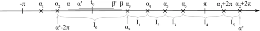
-π α₁ α₂ α α' t₀ β' βα₃ α₄ α₅ α₆ π α +2π α +2π_{1 2}

I I I I I I

0 1 2 3 4 5

α -2π* α_* α^*

Figure 1: Prescribed zeros and intervals in the trigonometric case Remark: Note that (the second half of) (9) implies (11).

We need the following trigonometric form of fast decreasing polynomials. In the proof we use so-called half-integer trigonometric polynomialsPn

j=0a_jcos((j+

1/2)t)+b_jsin((j+1/2)t). They are natural in this context, see, e.g. the product representation [2], p. 10, or Videnskii’s original paper [30], or the paper [16].

Theorem 3. Let t0, α, β, α⁰, β⁰ ∈ (−π, π) be such that −π < α⁰ < α < t0 <

β < β⁰< π andα1, . . . , αl∈(−π, π)\[α⁰, β⁰] be with the corresponding positive integer powersk1, . . . , kl. PutZ(t) :=Ql

j=1

sin^t−α₂^j

kj

.

Then there existsδ1>0such that for all largemthere exists a trigonometric polynomialQmwith degree at most msuch that

Q_m(t₀) = 1, (20)

0≤Qm(t)<1 fort∈[−π, π), t6=t0, (21) Q^(k)_m (α_j) = 0, j= 1, . . . , l, k= 0,1, . . . , k_j, (22) Qm(t)≤min(1,|Z(t)|) exp(−δ1m)fort∈[−π, π]\(α⁰, β⁰), (23)

|Qm(t)−1| ≤exp(−δ1m)fort∈[α, β], (24) Q_m(t)is strictly monotone on [α⁰, α]and on [β, β⁰]. (25) Proof. Briefly, we use similar idea as in the previous proof (Theorem 2), but there are lots of differences.

First, we introduce the intervals between the neighboring α_j’s as follows using the ordering ofαj+j2π, j = 1, . . . , l, and j = 0 if αj > β⁰ and j = 1 otherwise. Let Ij’s, j = 1, . . . , l−1 denote the closed intervals such that endpoints are the αj+j2π’s and they are disjoint except for the endpoints, and they are ordered from left to right (that is, ift1∈Ij andt2∈Ikandj≤k, thent1≤t2). Denote the left endpoint ofI1 byα_∗, and the right endpoint of I_l−1 byα^∗, that is, α_∗ andα^∗ are the minimum and maximum ofαj+j2π’s respectively. PutI0:= [α^∗−2π, α∗], this wayI0, I1, . . . , Il−1 cover an interval of length 2πandt0∈I0, [α⁰, β⁰]⊂I0. Note thatIj’s are not necessarily subsets of (−π, π).

We define Z˜1(t) :=

l

Y

j=1

sint−αj

2 k⁰_j

, R(τ;˜ t) = ˜R(t) :=

l−1

Y

j=1

sint−τj

2 , P˜0(t) = ˜P0(a, µ;t) :=

cost−a 2

2µ

, P˜₁(a, b, λ, µ;t) = (1−λ) ˜P₀(a, µ;t) +λP˜₀(b, µ;t)

where k_j⁰ =k_j ifk_j is even and k_j⁰ =k_j+ 1 if k_j is odd, for j = 1, . . . , l, and τ_j ∈ I_j, j = 1, . . . , l−1, and α⁰ < a < α < β < b < β⁰, a := (α+α⁰)/2, b:= (β+β⁰)/2, andλ∈[0,1]. We also putk₀⁰ =k₀ifk₀is odd andk⁰₀=k₀+ 1 ifk0 is even; and τ := (τ1, . . . , τ_l−1). As above, if some of the parameters are fixed or unimportant in the current consideration, then we leave them out, e.g.

P˜0(t) = ˜P0(a, µ;t) and ˜P1(t) = ˜P1(µ;t) = ˜P1(λ, µ;t) = ˜P1(a, b, λ, µ;t).

Some immediate properties are the following: Z(t), ˜˜ P0(t) and ˜P1(t) are nonnegative trigonometric polynomials. Ifl is even, then ˜R(t) is a half-integer trigonometric polynomial, iflis odd, then it is a trigonometric polynomial (with degree (l−1)/2).

Consider

S˜1(t) := ˜Z1(t) ˜P1(µ, λ;t) ˜R(τ;t)

sint−t0

2 k₀⁰

which is a trigonometric polynomial iflis even and is a half-integer trigonometric polynomial iflis odd. We need

S˜₂(t) :=

(S˜1(t), iflis even, S˜1(t) cos^t−(α₂^∗−π), iflis odd which is a trigonometric polynomial in both cases.

Now we would like to integrate ˜S1(.) and get a trigonometric polynomial too. To do this, we use Poincar´e-Miranda theorem, as in the proof of Theo- rem 2. Consider the rectangleR := [0,1]×I₁×I₂×. . .×I_l−1 and (λ, τ) = (λ, τ₁, . . . , τ_l−1)∈ R. We use the functions

fj(λ, τ) :=

Z

Ij

S˜2(λ, τ , µ;t)dt, j= 0,1, . . . , l−1.

Note that sin^t−t₂⁰ is negative on (α^∗−2π, t0) and is positive on (t0, α^∗), cos^t−(α₂^∗−π) is positive on (α^∗−2π, α^∗) but it introduces an extra zero atα^∗. It can be ver- ified same way as in the proof of Theorem 2 that there are sign changes inf0

as λchanges from 0 to 1, and in fj as τj goes from the left endpoint ofIj to the right endpoint ofIj.

Poincar´e-Miranda theorem shows that there are particular λ∈ [0,1], τ1 ∈ I1, . . . , τ_l−1 ∈I_l−1 such that all thefj’s are zero; fix this solution and denote

it byλ, τ1, . . . , τ_l−1in the rest of this proof. Summing up these integrals for all j= 0,1, . . . , l−1, we also obtain that Rα^∗

α^∗−2πS˜2(t)dt= 0.

Put

S(t) :=˜ Z t

α∗

C1S˜2(τ)dτ

where C₁ will be chosen later (like in the proof of Theorem 2). In both cases (l is even or odd), the integrand is a real trigonometric polynomial. Since the integral of ˜S₂(t) over [α^∗−2π, α^∗] is 0, ˜S(t) is also a trigonometric polynomial.

C1 can be chosen so that

Z t₀ α∗

C1S˜2(t)dt= 1

holds. The properties (20), (22), (23), (24) and (25) can be verified same way as in the proof of Theorem 2. A key tool was the Nikolskii inequality for algebraic polynomials and it should be replaced with the similar inequality for trigonomet- ric polynomials, which is again due to Nikolskii (see, e.g [14], p. 495, Theorem 3.1.1). Again, squaring ˜S, we can construct the trigonometric polynomial which also satisfies (21).

3.2 Rough Markov- and Bernstein-type inequalities

The following two propositions have rather simple proofs, they may be known, but we could not find reference for them.

Proposition 4. Let I ⊂ (−π, π) be a closed set consisting of finitely many disjoint intervals such that none of them is a singleton and k be a positive integer. Then there exists C = C(I, k) > 0 such that for all trigonometric polynomialTn with degreen, we have

T_n^(k)

_I ≤Cn^2kkTnk_I. (26) This immediately follows from iterating Videnskii’s inequality on each com- ponent (maximal subinterval) of I. For Videnskii’s inequality, see [2], p. 243 (Exercise E.19 part c]) or [31].

We also need a rough Bernstein-type inequality for higher derivatives of trigonometric polynomials.

Proposition 5. Let I ⊂ (−π, π) be again a closed set consisting of finitely many disjoint intervals such that none of them is a singleton andkbe a positive integer. Fix a closed setI₀⊂IntI(subset of the one dimensional interior ofI).

Then there existsC=C(I, I0, k)>0such that for all trigonometric polynomial Tn with degreen, we have fort∈I0

T_n^(k)(t)

≤Cn^kkTnk_I. (27) This again, immediately follows from applying Videnskii’s inequality (see [2], p. 243, E.19 part b]) iteratively on the component (sayI₀⁺) ofI containing I₀ and finally usingkT_nk_I+

0 ≤ kT_nk_I.

3.3 Asymptotically sharp Markov-type inequality

Theorem 6. Let E ⊂(−π, π)be a compact set satisfying (2). Then for any trigonometric polynomialT_n with degreen, we have

T_n^(k)

_[a−ρ,a]≤(1 +o(1))n^2kΩ(E_T, e^ia)^2k 8^kπ^2k

(2k−1)!!kTnk_E (28) whereo(1)is an error term that tends to0asn→ ∞, depends onEanda, but it is independent of Tn. This inequality is sharp, that is, there is a sequence of trigonometric polynomialsTn,n= 1,2, . . ., such that degTn=nand

T_n^(k)(a)

≥(1−o(1))n^2kΩ(E_T, e^ia)^2k 8^kπ^2k

(2k−1)!!kTnk_E, (29) whereo(1)→0 is an error term depending onE andn.

Proof. The proof of (28) is divided into five steps and then (29) will be estab- lished.

First step. We prove the assertion whenEis a T-set, andT_nis polynomial of the defining polynomialU_N for this set. That is,E={t∈(−π, π) : |UN(t)| ≤ 1} (as in (4)) and there is a real, algebraic polynomial P such that T_n(t) = P(U_N(t)). We may assume thatU_N(a) = 1 (we know that|U_N(a)|= 1).

Now we use Fa`a di Bruno’s formula (1). Note that, in our setting f = P (outer function) andg=UN (inner function), hence the product is independent ofP andn(andTn too). Hence we reorder the terms decreasingly:

(P◦UN)^(k)(a) =P^(k)(1) (U_N⁰ (a))^k+. . . (30) where in the remaining terms onlyP^(k−1)(1), P^(k−2)(1), ... P⁰(1) occur. There are finitely many remaining terms and by (26), they grow liken^2k−2asn→ ∞.

As for the first term, we can use the classical V. Markov inequality (see e.g. [2], p. 254) andkPk_[−1,1]=kTnk_E, hence withd:= deg(P),

|P⁰(1)| ≤ d²(d²−1). . . d²−(k−1)²

(2k−1)!! kTnk_E ≤d^2k 1

(2k−1)!!kTnk_E where actually

d²(d²−1). . . d²−(k−1)²

d^2k →1 (31)

asn→ ∞(which is equivalent tod→ ∞).

As forU_N⁰ (a), we use the density of the equilibrium measure, more precisely formula (3.21) from [28] (anda=a2j0), hence

|U_N⁰ (a)|= 2N²

Qm l=1

e^ia−e^iτl

2

Q

l=1,...,2m,l6=2j0|e^ia−e^ial| = 2N²Ma,k= 8π²N²Ω(E_T, e^ia)². (32)

Putting these together:

T_n^(k)(a)

≤(1 +o(1))8^kπ^2k 1

(2k−1)!!Ω(E_T, e^ia)^2kn^2kkTnk_E.

Now we extend the previous inequality from a to [a−ρ, a] (as in (28)).

Basically we use the smaller growth of the rough Bernstein-type inequality (27) and the continuity of U_N⁰ . For any ε > 0, we can select η > 0 such that [a−η, a]⊂Eand fort∈[a−η, a] it is true that

|U_N⁰ (t)| ≤(1 +ε)|U_N⁰ (a)|= (1 +ε)8π²N²Ω(E_T, e^ia)². Then fort∈[a−η, a] we get from (30) and again from (26) that

T_n^(k)(t)

≤(1 +o(1))(1 +ε)8^kπ^2k 1

(2k−1)!!Ω(E_T, e^ia)^2k n^2kkTnk_E. (33) Now, on [a−ρ, a−η] (if not empty), we can use the rough Bernstein-type inequality (27), hence we obtain an upper estimate forT^(k)(t) which has growth ordern^k, which is smaller thann^2k, the growth order of the Markov factor. So if nis large (depending onε), then (33) holds fort∈[a−ρ, a−η] too. Now letting ε→0 appropriately, (28) follows forT_n(.) =P(U_N(.)) asd= deg(P)→ ∞.

Second step. Now we establish (28) whenE is a T-set and T_n is arbitrary trigonometric polynomial. We use symmetrization here (see, [25] pp. 151-152 and [28], pp. 2997-2998, including Lemma 3.2) and fast decreasing trigonometric polynomials (see Subsection 3.1). In this step we work in a smaller neighborhood ofa, i.e. on [a−ρ₀, a] where ρ₀< ρis defined later.

Letj0 correspond to the interval in whichais. More precisely, sinceE is a T-set in this case, there are 2N disjoint, open intervals such thatUN maps these intervals to (−1,1) in a bijective way. Let us label them byEj = (α_2j−1, α2j) where −π < α1 < α2 ≤ α3 < α4 ≤ . . . ≤ α2N−1 < α2N < π. Hence a ∈ [α2j₀−1, α2j₀] and by (2),a=α2j₀. Put ρ0 := 1/4 min(α2j₀ −α2j₀−1, α2j₀+1− α2j₀, ρ, π/4).

We also need the following facts on T-sets. SinceUN(.) is 2N-to-1 mapping, we need its restricted inverses. Let U_N,j⁻¹(t) be the inverse of UN restricted to [α2j−1, α2j] and put tj(t) = tj := U_N,j⁻¹(UN(t)). Obviously, tj is C^∞ on

∪^N_j=1(α_2j−1, α_2j) and now we give estimates for the l-th derivative of t_j(t), especially, ast approachesa. Similarly, as in [23], if l= 1 orl= 2, then

dtj

dt = d

dtU_N,j⁻¹(UN(t)) = U_N⁰ (t)

U_N⁰ (U_N,j⁻¹(U_N(t))) = U_N⁰ (t) U_N⁰ (tj), d²

dt²U_N,j⁻¹(U_N(t)) = −(U_N⁰ (t))²U_N⁰⁰(U_N,j⁻¹(UN(t)))

U_N⁰ (U_N,j⁻¹(UN(t)))³ + U_N⁰⁰(t) U_N⁰ (U_N,j⁻¹(UN(t)))

=−(U_N⁰ (t))²U_N⁰⁰(tj)

(U_N⁰ (t_j))³ + U_N⁰⁰(t) U_N⁰ (tj)

and for generall, Fa`a di Bruno’s formula (1) implies that there is a universal polynomialQl(independent ofUN, depending onl only) which is a polynomial inU_N^(k)(t) andU_N^(k)(tj)k= 1, . . . , l, that isQl=Ql(. . . , U_N^(k)(t), . . . , U_N^(k)(tj), . . .) such that

d^l

dt^lU_N,j⁻¹(UN(t)) = Ql

(U_N⁰ (tj))^2l−1. (34) Here,Qlis independent ofnandTn, hence|Ql| ≤Cfor someC=C(k, UN)>0.

Moreover, we need to estimate|U_N⁰ (tj)|ast→aand we split the argument into two cases. Ifj is such thataj ∈IntE, that is,U_N⁰ (aj) = 0, and using that all the zeros of UN are simple, we can infer that U_N⁰⁰(aj) 6= 0, so |U_N⁰ (tj)| ≥ O(|tj −aj|). On the other hand, if j is such that aj ∈ E \IntE, that is, U_N⁰ (aj)6= 0, then simplyU_N⁰ (tj)≈U_N⁰ (aj). Hence, in any case

|U_N⁰ (tj)| ≥O(|tj−aj|). (35) For an arbitrary polynomialTn considerVn(t) =L^√_n(t)Tn(t), whereL^√_n(.) denotes the fast decreasing polynomial which has the following properties. L^√_n(.) has degree at most √

n, it is a fast decreasing trigonometric polynomial and peaking at a very smoothly (that is, L^√_n(a) = 1 and L^(j)√_n(a) = 0, j = 1,2, . . . ,2k²),L^√_n(.) is approximately 1 on [a−ρ₀, a+ρ₀] and is approximately 0 outside [a−2ρ₀, a+ 2ρ₀] and vanishes at the other extremal points ofU_N up to order 2k² (that is, ifUN(t) =±1,t6=a, thenL^(j)√_n(t) = 0, j= 0,1, . . . ,2k²).

Such polynomialL(.) =L^√_n(.) exists because of Theorem 3.

For simplicity, put W(t) := Q

j

sin^t−α₂^j2k

where j = 1, . . . ,2N, j 6=j0. ThisW is a nonnegative trigonometric polynomial and has sup norm at most 1. There is another trigonometric polynomialY(.) such that

L(t) =Y(t)W^k(t).

The sup norm ofY over [−π, a−ρ₀]∪[a+ρ₀, π] can be estimated using (23) withW^k in place ofZ. Hence, fort∈[−π, a−ρ₀]∪[a+ρ₀, π]

|Y(t)|=

L(t) W^k(t)

≤min 1

W^k(t),1

exp (−(degL)δ1). DifferentiatingL(.)j-times,j= 0,1, . . . , kwe write

L^(j)(t) =

j

X

l=0

j l

Y^(j−l)(t) W^k(l)

(t). (36)

Here W^k(l)

(t) = W(t)·. . . where W(t) is multiplied with other terms de- pending on W, W⁰, . . . , W^(l), k and αj’s only, and it is independent from n and Tn. As regards Y^(j−l)(t), we can use Videnskii’s inequality for Y(.) on

[−π, a−ρ0]∪[a+ρ0, π] (which is actually an interval on the torus), so there exists aC >0 such that for allt∈[−π, a−2ρ0]∪[a+2ρ0, π] and alll= 0,1, . . . , j

Y^(j−l)(t)

≤C(degY)^j−lexp (−(degL)δ1). (37) Summing up these estimates as in (36), we can write with degL≤√

n

L^(j)(t)

≤CW(t)n^j/2exp −√ nδ1

(38) whereC >0 is independent ofnandTn andt∈[−π, a−2ρ0]∪[a+ 2ρ0, π].

ThisVn has degree at mostn+√

nand satisfies kVnk_E ≤ kTnk_E,

Vn(t) =

1 +O(β

√n)

Tn(t) fort∈[a−ρ0, a],

|Vn(t)|=O(β

√n)kTnk_E fort∈E\[a−2ρ₀, a]











(39)

whereβ= exp(−δ1)<1.

Now, (by Leibniz formula), for alll= 1, . . . , k V_n^(l)(t)−T_n^(l)(t) = L^√_n(t)−1

T_n^(l)(t) +

l

X

j=1

l j

L^(j)√_n(t)T_n^(l−j)(t). (40) Using the rough Markov-type inequality (26), there exists a constant C = C(E, k)>0 such that for all 1≤j≤k, t∈E

L^(j)√_n(t)

≤C√

n^2j L^√_n

E=Cn^j,

T_n^(j)(t)

≤Cn^2jkTnk_E

and ift∈E\[a−2ρ, a], then applying (26) forL^√_n onE\[a−2ρ, a], we can write

L^(j)√_n(t)

≤C√

n^2j L^√_n

E\[a−2ρ,a]=Cn^jβ

√n. (41)

These imply that forl= 1, . . . , k

V_n^(l)(t)−T_n^(l)(t) =O

n^2lβ

√n+n^2l−1

kT_nk_E, t∈[a−ρ, a] (42)

and

V_n^(l)(t)

=O

n^2lβ

√n

kTnk_E, t∈E\[a−2ρ, a].

Define the ”symmetrized” polynomial as T^∗(t) :=

N

X

j=1

Vn(tj).