Dynamic Relocation of Emergency Ambulance Vehicles Using the AVL Component of the GPS/GPRS Tracking System
Čedomir Vasić
1, Bratislav Predić
1, Dejan Rančić
1, Petar Spalević
2, Dženan Avdić
31 Department of Computer Science, Faculty of Electronic Engineering, University of Nis, Aleksandra Medvedeva 14, 18000 Niš, Serbia
E-mail: cedomir.vasic@elfak.ni.ac.rs, bratislav.predic@elfak.ni.ac.rs, dejan.rancic@elfak.ni.ac.rs
2 Faculty of Technical Sciences, University of Priština, Knjaza Miloša 7, 38220 Kosovska Mitrovica, Serbia, E-mail: petar.spalevic@pr.ac.rs
3 State University of Novi Pazar, Vuka Karadžića bb, 36300 Novi Pazar, Serbia, E-mail: dzavdic@np.ac.rs
Abstract: Data concerning the routes of ambulance vehicles extracted from the database of an AVL system is used in this paper to compute the locations where these vehicles should be parked during the "waiting for a call" time. A modular algorithm based on the AVL component of the GPS/GPRS tracking system and a suitable approach in resolving a mathematical problem, known as the "p-median", are proposed. The implemented solution of the redeployment problem is tested on the site.
Keywords: AVL; EMS (Emergency Medical Service); vehicle relocation; p-median
1 Common Conditions and Goal
Allocation and redeployment problems in resources management have been resolved in various ways many times in multiple fields of research. The development of the spatial model based on GIS (Geographical Information System) using the advanced AVL (Automatic Vehicle Location) component of the GPS/GPRS (Global Positioning System / General Packet Radio Service) tracking devices allow for new opportunities in deployment optimization. With the
additional computational power available to researchers, it is possible today to efficiently analyze the data generated by the GPS/GPRS-trackers. Software involved in the AVL component of the system allows dynamic analysis and an optimal decision making process. Allocation and redeployment problems are similar for any fleet of vehicles in all fields of transportation. Commonly, researchers focus on problems of planning services in the public sector.
Emergency Medical Services (EMS) and the fleet of ambulance vehicles are especially interesting because of their nature and the requirement of minimal response time. In papers related to the planning and organization of the EMS, allocation and redeployment are only a part of the extensive problems set. The approach to the process modeling and algorithm development is significantly influenced by the available input data and the available resources, though the main goal is always same: to reach a patient as soon as possible. Models used in system designing processes differ in approach. The prerequisites researchers encounter vary from: how many vehicles are the minimum requirement for functional service, how many vehicles are needed for a service to be functional at any moment, where garages need to be placed to minimize reaction time, etc. During the operation of the established EMS, after any single call for intervention is received, a couple of important decisions have to be made: which vehicle to use (which vehicle is allocated) and were to locate the parking place for the vehicle in the status of “waiting for a next call” (relocation of vehicle). The relocation problem is simplified because we need to the find location with the best spatial coverage that provides the shortest time of response.
2 Problem Definition
Our work is targeted at the optimization of the existing EMS. The experimental part of the research is performed on an existing emergency vehicle AVL system that has been in use for a couple of years. All ambulance vehicles are equipped with GPS/GPRS tracking devices, and the appropriate software is installed in the control center. The input data we used in our research are limited to data available in the archive generated by the AVL component of the software over a prolonged period of time. The available data comprises the location coordinates, speed, date and time collected from vehicles in the EMS fleet of the ambulance vehicle in the city of Niš, Serbia.
After performing extensive analysis of the collected data, we propose a solution for the relocation of the ambulance vehicles during the "waiting for a call" time.
Emergency service is treated in a dynamic way, and the ambulances are relocated once every day. The main contribution of this project is one more options in the AVL software. The options are intended to be a useful tool available in the decision making process conducted by the dispatcher in the "call center". The
route history of the ambulance vehicles and the spatial locations of incoming calls, acquired from the AVL system are good starting points in resolving a relocation problem. If we can perform data analysis and recalculation of the optimal vehicle waiting locations at any time, we can achieve the goal, and we can provide a tool for the dynamic relocation of available recourses in EMS. Although the goal of finding the quickest route to the destination is impacted by many complex parameters, it is mainly influenced by Euclidian distance. Traffic jams, rush hours, road reconstruction, weather conditions, time of the year and other parameters also have to be taken into count when modeling dynamic allocation. In our case, we made the assumption that an ambulance vehicle can be parked and "wait for a call" at any location from which a call for service was received in the previous 30 days. We assume that the response time is mainly influenced by the distance between two points.
3 Previous Studies
3.1 Static or Dynamic Approach in Service Design
The direction taken during modeling mainly depends on whether we are designing a service from scratch or we are optimizing and evaluating an existing service.
Depending on that decision, we can treat a service as static or dynamic. If the goal is to find a minimal number of vehicles necessary to meet the required coverage or required average time of response, we are treating the service as a static one. In that case, we resolve the problem once, in the beginning of a service design. If we want to use new technologies and improve the existing service by introducing new procedures, the service is treated as a dynamic one. In this case, the everyday routine is changed daily and existing resources are used in a more efficient and productive way. The third approach is used in the case of the evaluation of an existing service. A model dedicated to the quality of the service control and quality assessment is sometimes required as a tool in a future investment planning.
Among the first successful solutions was a model proposed by Church and ReVelle [1]. This model, named the “Location Set Covering Model” (LSCM), was dedicated to minimizing the number of facilities required to cover required service distances. This model is useful only if one wants to find the minimum number of necessary ambulance vehicles to provide a required service level. The authors note that an unlimited number of ambulance vehicles is not a realistic case and modified the proposed model into a new one named: “Maximal Covering Location Problem” (MCLP). The new model aims to maximize the population coverage by the limited ambulance usage. Soon, it was identified that if one of the vehicles is on the way and another incoming call occurs in the region subordinated to that
vehicle, the new demand will not be served in the specified time limits. So a whole group of new models was developed under common name: Double Standard Models (DSM). One of them is proposed by Gendreau [2]; the model guarantees response to any incoming call by two vehicles in a defined time limit in the city of Montreal, Canada. After several years, Gendreau proposed a dynamic relocation of the ambulance fleet during the idle time between two incoming calls and named the new model “Dynamic Double Standard Model”
(DDSM). Gendreau defined the new problem as the “Maximal Expected Coverage Relocation Problem” (MECRP) and included a constraint of the number of redeployments. Researchers noticed that during one shift, one vehicle can serve only a limited number of the calls, and this model introduces the capacity of the vehicle. Malandraki i Daskin [3] turned to the probabilistic approach and assigned a “server busy probability” variable to ambulance vehicles. The proposed model is named the “Maximum Expected Covering Location Problem” (MEXCLP).
Schilling [4] resolved real life situations using several vehicle types and developed a model named the “Tandem Equipment Allocation Model” (TEAM) and later an extended version of the model named FLEET. Most of the recent work is based on well-known studies, and extensive effort was used in the examination of the differences and a comparison of the results.
3.2 Static or Dynamic Approach in Environment Modeling
The next important issue in modeling is related to the changing impact of the environment. Again, it can be approached both statically and dynamically.
Introducing time dependent functions as a representation of the model parameters represents dynamical modeling. This includes dependency related to the season of the year, day of the week, hour of the day, dependency related to the meteorological conditions, temperature, etc. Generally, this time dependency is introduced in the model by the time dependent average speed of the vehicle on the observed part of the drive track. Historical data provided by the modern GPS/GPRS vehicle trackers, especially data about vehicle speed, known as FCD (Floating Car Data) is a valuable input into such approaches. The TIMEXCLP model suggested by Repede and Bernardo [5] was among the first papers introducing environment impacts. The authors extended the already mentioned MEXCLP model into the TIMEXCLP model and applied a procedure on the data acquired in Louisville-Kentucky using variations in travel speed as a function of the time of day. The result was an increase of calls responded to within 10 minutes, from 84% to 95%. The MEXCLP model was criticized as treating all servicers with the same busy probability. Rajagopalan [6] defined a function for modeling the probability of a desired vehicle to be already occupied. For most of these models, it can be assumed that the environment is treated dynamically. It is taken into account that the time of the route from point A to point B varies during different periods of the day.
3.3 Examples of Integral Solutions Deployments
A review of the different practical solutions and their strengths is systematically examined by Kolesar [7]. This model was tested in New York, and for the first time, the possibility of redeployment of fire-units during one day shift was used.
Budge [8] presented a model field deployed in Calgary, Canada. FCD data on the vehicles’ speed obtained from the database connected to AVL software is used for the first time by Reinthaler [9]. Examples of an integral solution in optimization of the Emergency Medical Service in urban areas can be found in many large cities all over the world. Approaches to the problem definition and solution differ significantly for different cases. Population layout, road networks, data about traffic accidents, and insurance users’ addresses are commonly used.
3.4 Previous Work Related to the P-median Problem
We address a well-known optimization issue, which is in our case mathematically represented as a p-median problem. This problem was defined for the first time in papers by Hakimi [10]. He divided continuous space into a discrete network and assumed that medians can be placed at the graph vertices. He gives mathematical proof that there is at least one optimum solution of this problem. Finally, he proposed a simple enumeration procedure named “direct enumeration” for the calculation of one or more medians. ReVelle and Swain [11] provided the first linear programming formulation of the problem and involved integer variables in the numeric resolving. They proposed a “Greedy Adding Algorithm” and a modified version, the “Greedy Adding with Substitution”. These papers are the basis for all methods proposed later. For large values of n and p, direct enumeration is not an acceptable solution, and methods that provide approximate solutions are introduced. Methods known as heuristics are developed as two phase algorithms. The first phase always consists of finding a starting set of p-medians, and the second phase includes iterations dedicated to solution improvement. The final solution is commonly very close to the optimal one, and sometimes it is the optimal solution. There are three primary early heuristics: Greedy, Alternate and Vertex Substitution. The "Greedy" method is described in the works of Kuehn and Hamburger [12]. This method was dedicated to resolving the warehouse location problem. The problem is how to place p-warehouses and supply n customers with a minimal total cost. Teitz and Bart [13] defined a method known as “vertex substitution” or "interchange" heuristic. In this solution, they frequently use a common subroutine known as the “one-opt” procedure. The procedure is used to find the "first" median by exact calculations similar to looking for the total cost of a single node. Densham and Rushton [14] improved the “vertex substitution”
method and pointed to a spatial distribution of network nodes. They created a spatial search procedure as a more efficient and effective tool dedicated to the examination of possible solutions. This procedure is implemented as a core of the
new method called Global Regional Interchange Algorithm (GRIA). “Vertex substitution” is the most commonly used procedure in engineering practice.
The method known as Lagrange relaxation is introduced if determining the starting medians and direct enumeration as a method for the total cost calculation appears to be inadequate. We mitigate the starting constraints to the mathematical definition of the problem, and we introduce problem relaxation. Iterations are controlled in several different ways: sub gradient-relaxation or growing- optimization, brunch-and-bound, double-incrementing or “surrogate”
optimization, etc. The milestone work in this research branch includes the algorithm by Narula, Ogibu and Samuelsson [15]. The newest “Surrogate”
relaxation from Senne and Lorane [16] uses a new approach and uses a whole range of multipliers to improve the standard relaxation technique.
The most common metaheuristics are “Variable Neighborhood Search”, “Genetic Algorithms”, “Tabu Search”, “Heuristic Concentration”, “Simulated Annealing”
and “Neural Networks”. Hansen and Mladenović [17] developed a metaheuristic method named “Variable Neighborhood Search” (VNS). The algorithm is implemented in several steps. The first step is adopting an arbitrarily chosen starting solution. Starting nodes are randomly taken from network. After that, a procedure named "shaking" is applied, and one node in the solution is replaced with a new one, taken from the neighborhood. The quality of the new solution is examined and if the new solution is better than the previous one, the new solution is accepted as valid. Shaking is applied again, and the quality of the new result is checked. Systematic change of the neighborhood space is crucial. The process involves exploring increasingly distant neighborhoods to avoid a local minimum.
The quality of the whole algorithm is in direct correlation to the quality of the shaking method. Different methods are used, and the most common are:
"diversification" and "intensification". Practice proved VNS to be a very useful and convenient method. Thanks to different shaking methods, there are many variations of the original idea, such as “Parallel Variable Neighborhood Search”
(PVNS), “Cooperative Parallel Variable Neighborhood Search” (CPVNS), and
“Greedy Randomized Adaptive Search Procedure” (GRASP).
“Heuristic Concentration” is developed by Rosing and ReVelle [18]. If we randomly choose locations of the starting set, there is 20% probability of falling into a loop that leaves us far from the optimal solution. At same time, if we apply
"concentration", this risk is reduced to only 5%. The “Tabu procedure” involves such methods as restrictions, aspiration criteria, diversification and strategic oscillations. “Simulated Annealing” is one of the metaheuristics derived in attempts to use principles identified in nature as the template for mathematical algorithms. Mathematical implementation of cooling structures and achieving thermal equilibrium is used as a method for vertex substitution. Among the newest metaheuristics are “Genetic Algorithms” proposed for use in resolving the p- medianproblembyHosageandGoodchild [19],andlaterintheworks of Alp, Erkurt and Drezner [20].
4 Experimental Work
4.1 Common Issues in EMS
Emergency Medical Service (EMS) in the town of Niš, Serbia, is a public service organized to meet the needs not only of residents of downtown but also to residents of the 68 neighborhood settlements. The area of approximately 600 km2 contains more than 300.000 habitants, and these are serviced by 24 specialized ambulance vehicles and a dozen vehicles with specific and unique medical equipment. The fleet is relatively new and is well-equipped with up-to-date standard medical equipment. Four vehicles are always on duty with complete personnel, and these operate in 8-hour shifts.
If there are no incoming calls, vehicles are parked in a central garage near an emergency medical site, and the staff is resting in a leisure room. All other vehicles are also in a central garage parked for service, for recharging batteries, fuel filling, cleaning, etc. In addition to the 4 vehicles on duty,thereare5vehicles readytobeusedinanunpredictableextraordinarysituation.
The firstassumptionwemadeinthispaperisthatambulancevehiclesneednotwait in a centralgarage butcan be parkedin one ofthe parkinglocations arrangedto minimizetheaverage time of response. Every vehicle receives the coordinates of a designated parking location, and after finishing the previous intervention, they go directly to that location. A vehicle goesbacktothecentralgarageonlyattheendof the shift. Thewhole areaofthe cityhas to be divided into 4 regions, and each region is assigned to one vehicle.
4.2 AVL Component of the System and Impact on the Final Solution
The experimental part of the research conducted in this paper and the verification in practice relies on data collected by a unit named a "GPS/GPRS-tracker". These units include a GPS-receiver, GPRS-modem, microcontroller dedicated to synchronization of operations and local memory for storage of positional updates, assembled in one case. Memory is used in the case of restricted GPRS network coverage, preventing any positional data loss. In this case, real time ambulance visualization is not available, but no data are lost. Vehicles’ positions are recorded periodically, and updates are transferred to the server located at the control center using a GSM phone network and a GPRS packet data transfer service offered by a local mobile phone operator.
Each vehicle location is matched to the underlying road network and displayed over a city raster map acting as a background. The full vehicle trajectory during response to an emergency medical call is then reconstructed from road segments
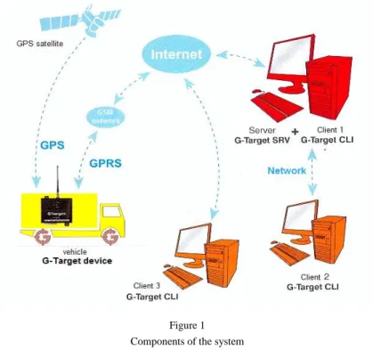
and stored as one instance of emergency response. Real time coverage and actual position of the whole fleet is available to all users according to granted permissions to connect to the server. The server provides updated picture in several resolutions adjusted to type and throughput of connection. Cell-phones, PDA-units and other devices are also supported. All components of the system with mutual dependencies are shown in Figure 1.
Figure 2 shows a snapshot of the application and actual location of an ambulance vehicle. This is a working environment for the dispatcher in the "calling center"
operated by the EMS. The AVL subsystem creates a new record in the database for every new position of ambulance vehicle. The records include following fields: vehicle identifier, location coordinates, time, direction, speed, etc. During the first execution phase of the algorithm proposed in this paper, destination points related to ambulance routes are separated from the extensive amount of positional data in the database.
Coordinates of destination points are just one parameter that can be used as query criteria. Other modules of the software are tasked with trip instance extraction by identifying the starting point, ending point and all points belonging to that specific trip instance. Each road segment can have a weight factor assigned that can be usedincalculations,butthispossibilityisnot usedatthistime.Trafficconditionsas aninput parameter for the arrival time estimation will be used in the future studies.
Figure 1 Components of the system
Figure 2
Vehicle fleet management application
4.3 P-median Problem Definition
If the main goal is to achieve a minimum average response time, then we use a model based on the p-median mathematical representation of the problem. If the goal is to achieve a minimum for the longest response time, then we use a model based on the p-center mathematical representation. The most important difference is the fact that the p-center model does not consider the weight of a location.
Using the p-center model, we try to reduce the longest travel time, and the number of incoming calls from the same location is not considered.
The problem of identifying p-facilities (called “medians”) to minimize the sum of distances for each client location to its nearest facility was defined during the early sixties as a p-median problem. The resolving of this problem is classified as a non- deterministic polynomial-time (NP) difficulty problem. For even moderate values of client points n and facilities p, the number of possible solutions can be very large and is defined by (1):
)!
(
!
! p n p
n p
n
. (1)
For instance, if n=1000 and p=10, the total number of possible solutions is 2.631.023,00. In this paper, the p-median problem is treated as a binary integer programming problem, explained as the following: find the minimum of (2):
iI jJ ij ijjd y
(2) where j is the weighting factor of location j, and dij is the Euclidian distance between location i of a parked vehicle and location j of an incoming call.
Particular constraints are assumed:
I i
i p
x (3)
J j y
I i
ij
,
1 (4)
J j I i x
yij i0, , (5)
i Ixi 0,1, (6)
i I j Jyij 0,1, , (7)
The constraint (3) defines that p is the total number of vehicles that we have to relocate, (4) says that one demand can be served by only one vehicle, (5) eliminates the possibility of serving a call from a location without a vehicle, (6) says that one parking place can contain only one whole vehicle (one vehicle cannot be divided into several locations) and in the end, (7) ensures that one incoming call can be serviced only by one vehicle (not with two halves of two different vehicles). Certain of the constraints can be removed or avoided, which is a relaxation of the problem. Additionally, some additional constraints can be introduced. For example, it is possible to define a maximum value for dij. This is a way to establish a maximum allowed call response time. Additionally, it is possible to introduce a maximum allowed number of calls serviced by one vehicle. This represents a capacity constraint.
5 Description of the Proposed Solution
5.1 Obtaining the Starting Solution
For the purpose of resolving the previously defined problem, a three phase algorithm is proposed. Coordinates of points of interest are extracted from the database connected to the AVL subsystem during the first phase. In the second
phase, a starting set of medians is calculated using direct calculations. In the third phase, the starting set of medians is improved using the Genetic algorithm. We start with a procedure dedicated to sequential search of the database, which contains all of the movement data of the ambulance vehicles. In the first phase of the algorithm, we examine data for the last 30 days for two ambulance vehicles arbitrarily chosen. The criteria for query are defined and implemented in a subroutine to traverse successive nodes on a path and to provide answers to questions like: “Is the vehicle moving?” or “Has the vehicle reached the destination?” Based on these answers and predefined constraints, nodes that are destinations of routes are extracted, and other nodes are ignored.
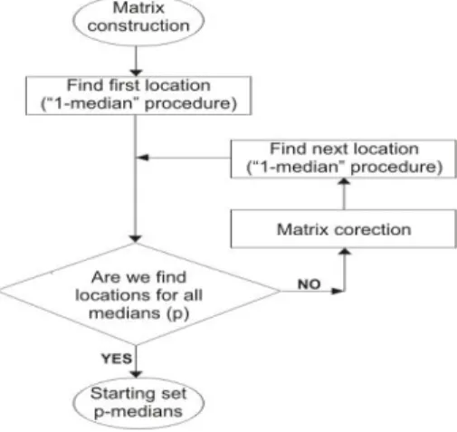
Figure 3 Algorithm flowchart
As a result of the first phase of the algorithm, we obtain locations as destinations in the observed period of time. Extracted nodes are sequentially searched again, coordinates are converted into integer data type and weight factors are assigned to each node. The criterion to join two incoming call nodes into one and to use a weight factor of 2 is that the distance between them is less than 60 meters. The second phase of the algorithm is shown as a flowchart in figure 3. The goal of this part of the algorithm is to provide a starting set of medians as a starting solution.
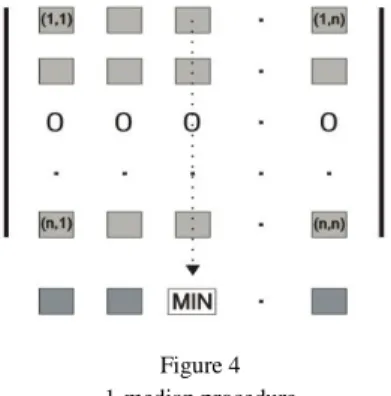
We construct an n x n matrix of distances and introduce a weight factor. The matrix consists of i-rows and j-columns. Element dij represents the distance from the incoming call node j to the parking location i multiplied by j (weight factor of node j). We apply a "1-median" procedure to the matrix. This procedure finds the most suitable parking location if we have only one vehicle.
Figure 4 1-median procedure
The "1-median" procedure is depicted in Figure 4. The third column is an array of distances to all other n – incoming call nodes according to the presumption that we always start from the parking place located at node number “3”. The sum of all elements placed in the third column of the matrix is the total distance we have to travel if we want to serve all incoming call nodes, and each time we start from the location of node number “3”. This sum is a measure of the quality of location number “3”, and we use this sum to compare the cost of that location to the costs of other locations. We calculate this sum for every column of the matrix and compare the costs of all the nodes and look for a minimum. The array of recalculated node costs is represented as the last gray row below the matrix in Figure 4. Column number "3" is designated as "MIN" because that column has the lowest cost. This means, in this hypothetical case, if we had only one ambulance, that vehicle should be parked in the location defined by the coordinates of node
"3". Node "3" is the first median of our matrix. The flowchart in Figure 3 represents the first iteration. Of course, the cost of node number “3” will not remain unchanged through further calculations because that cost will be influenced by introducing other medians.
If we have no more vehicles, the second phase of the algorithm should finish here.
However, because we have more vehicles, we fill the third row with zeroes, as represented in Figure 4, according to the fact that if we start from any location and the destination is node “3”, we need to travel zero kilometers to reach it because we already have a vehicle in that node. In the adjusted matrix, we apply the “1- median” procedure again to find the second median. The flowchart in Figure 3 represents this as the branch returning to the beginning of the algorithm. When the total number of the parking locations is exhausted, the second phase of our algorithm is complete. As a result, we have a starting set of medians. At the end of this phase, we sum all costs of the determined locations and obtain the total cost of the complete solution. It will be used in the future as a measure of solution quality for comparison with other solutions obtained in the future. A starting set of the medians is far from the optimal solution, and considerable work is required to improve it.
5.2 Basic Principles of Genetic Algorithms
Genetic algorithms are a family of computational techniques inspired by the mechanics of natural evolution, according to the Darwinian theory of natural evolution. These algorithms encode problems and solutions to a chromosome like data structure and apply evolution-like operators to these structures.
Implementation of a genetic algorithm begins with a definition of the search space as a finite bounded domain. The crucial step is determining a fitness function, according to the fact that in any point of search space, the value of the fitness function indicates the amount of closeness to the optimal solution. In many cases, using Genetic algorithm implementation is as good as the fitness or evaluation function. The next step is the initialization or selection of the initial population.
Through the next generations of the population, the existing solution is iteratively improved.
Genetic operators are needed to provide a searching mechanism for the algorithm.
These operators are used to create new solutions, and they are based on the existing solutions in the population. Two basic operators are crossover and mutation. Crossover takes two individuals, called parents, which are combined to form new chromosomes, called offspring. Iteratively applying the crossover operator, genes of good chromosomes appear more frequently in the population, leading to convergence to the optimal solution. The mutation operator alters one individual to produce a single new solution. Mutation introduces random changes into the characteristics of chromosomes. Mutation is generally applied at the gene level and introduces genetic diversity in the population, providing a way to escape from local optima. Reproduction involves the selection of chromosomes for the next generation. In general, the fitness of an individual determines the probability of its survival to the next generation. There are many different selection procedures, including roulette wheel selection, scaling techniques, tournament, elitistic and ranking methods. There are many types of Genetic algorithms according to different approaches to the population, reproduction and use of operators. The most commonly used are: standard, solid state, incremental, parallel, elitistic, niched, meta-level, and fuzzy. The benefits of using Genetic algorithms are numerous. The main benefits are: modular design, design separated from application, supported multi-objective optimization, easy adaptation to "noisy" environments, easy implementation, parallel processing, answers obtained quickly, answers are better as time goes by, many ways to speed up and improve application, and possibility to make combinations with hybrid solutions. The main disadvantage of the Genetic algorithm is the long computational time, but it can be terminated at any time. Sometimes longer runs are acceptable, especially with faster computers.
5.3 Components of the Genetic Algorithm Related to the Proposed Solution
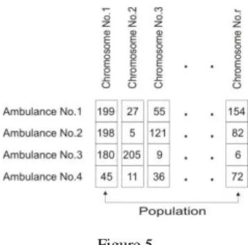
Chromosome coding is critical in terms of its ability to represent all possible solutions and to avoid introducing infeasible solutions in new populations. There are two possible representation schemes for chromosome coding: binary and non- binary. For our solution, we chose a non-binary representation in the following manner: a chromosome corresponds to a particular solution of our task. The length of a chromosome corresponds to the number of available ambulances. The locus of the first gene is reserved for ambulance number "1", and the last locus in the chromosome is reserved for the last ambulance vehicle. The serial number i of n possible candidate locations for parking places relates to a certain vehicle being placed in a corresponding locus. So we have p genes in one chromosome. In the locus of the first gene, we enter the number of the candidate location for the parking place assigned to ambulance No.1. The structure of the chromosomes is shown in Figure 5.
Figure 5 Chromosomes structure
The fitness function is the same as the objective function defined in the integer programming model (2). We calculate the total cost for every candidate solution from the distance matrix designed in the first phase. The sum of p costs of destinations included in the candidate solution is the total cost of the solution and a measure of the quality assigned to that solution. A smaller sum means a better fitted solution. Although the evaluation function may differ from the fitness function, in our case, they are identical.
Initial population. Having a wider initial population is a way to increase the probability of forming the best individuals. However, a wider population slows down the algorithm because we have to cultivate more chromosomes in every iteration. The objective is to find the optimal population size in which every possible solution can be attained through the genetic operators. The population size is related to the ratio between the total number of candidate locations and the total number of available vehicles. This ratio is named the "density" of the problem, and this concept
is developed in the widely cited paper of Alp, Erkurt and Drezner [45]. The proposed formula applied to our illustrative example case gives: 3*(n/p) = 162 as the desired number of chromosomes in the population. After population size is determined, the next step is to initialize the population. The first 10% of chromosomes in the initial population will be multiplied by the unchanged solution delivered from the second phase of our overall algorithm. The same starting chromosome is copy-pasted until 10% of population is initialized. The rest of population is filled with chromosomes randomly generated. Every gene as a candidate location is chosen randomly from the pool of i possible destinations.
Simultaneously, we take care about the feasibility of the solution and only chromosomes that meet the starting constraints are accepted. At the same time, we start to build a pool of already tested candidate solutions. If a chromosome is already accepted as part of the population, the procedure skips that candidate and asks for a new one.
Selection of parents. In the canonical genetic algorithm, the probability that two chromosomes will be selected for mating is proportional to their fitness. A common technique is mapping the population onto a roulette wheel, where chromosomes are represented by a space on the wheel surface. The amount of space proportionally corresponds to the chromosome’s fitness. In our case, before evolution starts with the new population, 10% of the best fitted chromosomes are directly copied from the previous population into the new population. This is the way to ensure that good genetic heritage is carried on to the next generation.
Parents are selected uniform-randomly from the population, and every individual has the same chance to be selected for the crossover. Although convergence to the best value is slower this way, this method increases the genetic diversity.
Crossover. With selected parents mated for crossover, we start recombination.
The recombination point is generally on 50%-60% of each chromosome, depending on the chromosome length. Swapping the fragments between two parents produces offspring. As we obtain two new chromosomes, first we check for feasibility and fitness. Better chromosomes continue further, whereas others are rejected.
Mutations. After recombination, a mutation operator is applied. A randomly chosen locus in the chromosome is replaced with a randomly chosen destination node. We check for feasibility again. At this point, we check if this chromosome was already examined as a possible solution. If this is not the case, the new chromosome finally becomes part of the new population.
Elitism in evolution. At the beginning of every new iteration, we build a new population from the old one. First, we recalculate the total cost of every chromosome in the old population and sort the chromosomes according to their fitness. Best fitted solutions are directly reinserted at the beginning of a new population.
Termination. A common practice is to terminate the Genetic algorithm after a predefined number of generations. It is also possible to terminate if the fitness of several top chromosomes remains unchanged for a predefined number of generations. In our example, we limited the algorithm to 200 iterations, but experiments confirmed that the algorithm always converges to an optimal solution after approximately 50 generations.
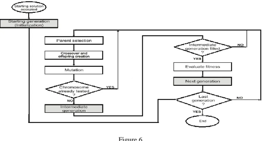
Algorithm iterations are shown in figure 6. The starting population is initialized partly with only one predefined chromosome multiplied to reach 10% of the population and partly with randomly generated chromosomes. The chromosome used for multiplication is the solution delivered from the second phase of the overall algorithm. During the process of evolution, while trying to reach a completely new population, we have to establish an intermediate population. After a fitness evaluation is applied, we copy the best 10% of chromosomes and fill the first 10%
of the intermediate population, whereas the rest of the chromosomes are generated using genetic operators. Mating, crossover and mutation are continuously repeated on the old population until the intermediate population is filled. At this point, the fitness evaluation is performed again to rearrange the chromosomes and sort the new population. At this point, it is easyto obtain thebest10%ofindividualsasthestarting pointofthenextintermediate population. To avoid unnecessarycomputation, we continuously store checked chromosomes in a poolof tested individuals, and every new candidate is compared with the contents of the pool. When a predefined number of generations is reached, the iterative process is stopped.
Figure 6 Algorithm iterations
5.4 Illustrative Example
We demonstrate our overall algorithm using an example based on real life data.
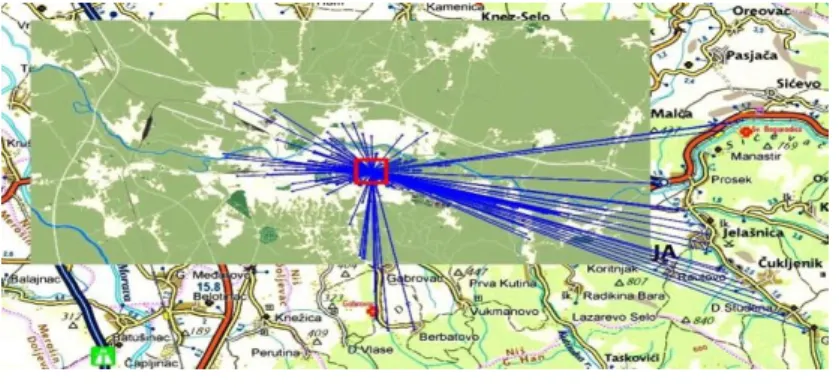
Figure 7 shows the complete history of routes driven by ambulance vehicle No. 1 over a period of 30 days. There is a total of 16.292 points in the AVL database,
which are used as the input data to our algorithm. Figure 8 shows the routes driven by ambulance vehicle No. 2 for the same period containing another 16.131 points.
Both histories were merged into one file, and the 32.423 points were used as input into the proposed first phase of the algorithm.
Figure 7
Complete route history for vehicle No.1 over 30 days
Figure 8
Complete route history for vehicle No.2 over 30 days
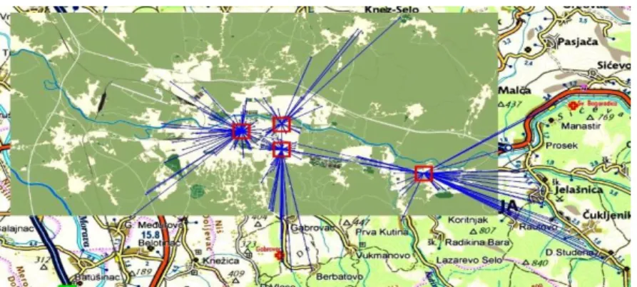
Figure 9 Results of the first phase
During the first phase of the algorithm, nodes are filtered, and nodes identified as destinations are extracted. From the 32.423 points, only 217 were identified as destinations. The appropriate weight factor is also determined and attached to every node. The results of this phase for ambulance vehicle No. 1 are shown in Figure 9.
As we can see on figure 9, the central starting point is the main garage of the EMS.
All destination nodes for vehicles No. 1 and No. 2 are merged into one array, enumerated from 1 to 217 and prepared for the second phase of the algorithm.
Figure 10
Proposed starting solution for the Genetic algorithm
Figure 11 Solution after 20 generations
Figure 12
Final solution after 50 generations
The second phase starts with the creation of the matrix of distances. Applying the
"1-median" procedure on the distance matrix, we generate the first possible solution. In our illustrative example, we assumed that there are 4 vehicles in one shift and that all of them are of the same type. The result is shown in Figure 10, and 4 locations can easily be identified as a proposed starting solution. The total cost of this solution is shown in Figure 13, as the cost of the best solution in the initial population (N = 0). After 20 generations, we have reached the data shown in Figure 11. The total cost of the solution reached after 20 generations can be identified on Figure 13. Figure 12 shows the solution after 50 generations, and this is our best total cost. The next 150 generations provides no improvement to the total cost.
Figure 13
Total cost of the solution reached after 20 generations
Conclusion
In this paper, we have proposed an innovative use of data collected using the AVL component of the GPS/GPRS tracking system for the optimization of emergency vehicle redeployment strategy. It is demonstrated that the use of developed GIS tools can significantly improve the quality level of emergency services in everyday routines. It is also applicable to all fields of public services and the transportation of people and goods. Practical results show that the Genetic algorithm with a calculated starting solution is a suitable tool for resolving the p- median problem in networks with less than a thousand nodes and less than a dozen medians. Verification and a practical testing process confirmed that the average
time needed to reach incoming call points was significantly less if vehicles were parked in the proposed parking places. The solution proposed in this paper is accepted as a standard routine in Emergency Medical Service in the town Nis, Serbia. Further improvements could incorporate an extra set of input data acquired from the AVL subsystem, such as the average speeds related to the road network segments or dynamic traffic congestion data.
References
[1] R. Church, C. ReVelle: The Maximal Covering Location Problem. Papers in Regional Science Vol. 32, No. 1, 1974, pp. 101-118
[2] M. Gendreau, G. Laporte, F. Semet: Solving an Ambulance Location Model by Tabu Search. Location Science Vol. 5, No. 2, 1997, pp. 75-88 [3] C. Malandraki, M. S. Daskin: Time-Dependent Vehicle Routing Problems:
Formulations, Properties and Heuristic Algorithms. Transportation Science Vol. 26, No. 3, 1992, pp. 185-200
[4] D. A: Schilling et al. The TEAM/FLEET Models for Simultaneous Facility and Equipment Sitting. Transportation Sci Vol. 13, 1979, pp. 163-175 [5] J. F. Repede, J. Bernardo: Developing and Validating a Decision Support
System for Location Emergency Medical Vehicles in Louisville, Kentucky.
European Journal of Operational Research Vol. 75, No. 3, 1994, pp. 567- 581
[6] H. K. Rajagopalan, C. Saydam, J. Xiao: A Multi-Period Set Covering Location Model for Dynamic Redeployment of Ambulances. Computers &
Operations Research Vol. 35, No. 3, 2008, pp. 814-826
[7] P. Kolesar, W. Walker, J. Hausner: Determining the Relation between Fire Engine Travel Times and Travel Distances in New York City. Operations Research Vol. 23, No. 4, 1975, pp. 614-627
[8] S. Budge, A. Ingolfsson, D. Zerom: Empirical Analysis of Ambulance Travel Times: The Case of Calgary Emergency Medical Services.
Management Science Vol. 56, No. 4, 2010, pp.716-723
[9] M. Reinthaler, B. Nowotny, F. Weichenmeier, R. Hildebrandt: Evaluation of Speed Estimation by Floating Car Data within the Research Project Dmotion. In: 14th World Congress on Intelligent Transport Systems, Beijing, China, 2007
[10] S. L. Hakimi: Optimum Locations of Switching Centers and the Absolute Centers and Mediansof a Graph, Operations Research, Vol. 12, No. 3, 1964, pp. 450-459
[11] C. ReVelle, R. Swain: Central Facilities Location. Geographical Analysis, Vol. 2, 1970, pp. 30-42
[12] A. A. Kuehn, M. J. Hamburger: A Heuristic Program for Locating Warehouses. Management Cience, Vol. 9, No. 4, 1963, pp. 643-666 [13] M. B. Teitz, P. Bart: Heuristic Methods for Estimating the Generalized
Vertex Median of Aweighted Graph. Operations Research, Vol. 16, No. 5, 1968, pp. 955-961
[14] P. J. Densham, G. Rushton: Designing and Implementing Strategies for Solving Large Location-Allocation Problems with Heuristic Methods.
Technical Report, National Center for Geographic Information and Analysis, Buffalo, NY, 1991, pp. 91-10
[15] S. C. Narula, U. I. Ogbu, H. M. Samuelsson: An Algorithm for the p- median Problem, Operations Research, Vol. 16, No. 5, 1968, pp. 955-961 [16] E. L. F. Senne, L. A. N. Lorena: Lagrangean/Surrogate Heuristics for p-
median Problems. In M. Laguna and J. Gonzalez-Velarde, editors, Computing Tools for Modeling, Optimization and Simulation: Interfaces in Computer Science and Operations Research, Kluwer Academic Publishers, 2000, pp. 115-130
[17] P. Hansen, N. Mladenović: Variable Neighborhood Search for the p- median. Location Science, Vol. 5, No. 4, 1997, pp. 207-226
[18] K. E. Rosing, C. S. ReVelle: Heuristic Concentration: Two Stage Solution Construction. European Journal of Operational Research, Vol. 97, No. 1, 1997, pp. 75-86
[19] C. M. Hosage, M. F. Goodchild: Discrete Space Location-Allocation Solutions from Genetic Algorithms. Annals of Operations Research, Vol. 6, 1986, pp. 35-46
[20] O. Alp, E. Erkut, Z. Drezner: An Efficient Genetic Algorithm for the p- median Problem. Annals of Operations Research, Vol. 122, 2003, pp. 21-42