Multisine Measurement Technology of Linearly Approximated Weakly Non-linear
Systems
Dissertation
Tadeusz P. Dobrowiecki candidate of the technical sciences
Budapest, 2016
Content
1. Introduction ... 3
1.1 The problem of the non-linear distortions ... 3
1.2 Overview of the literature ... 6
1.3 Research focus ... 7
1.4 Research assumptions ... 9
1.5 Summary of the scientific results ... 12
Jointly achieved research results ... 13
Contributions to the SISO theory ... 13
Contributions to the MIMO theory ... 16
1.6 Review of the content ... 18
2. General SISO theory ... 20
2.1 Problem introduction via simplified examples ... 20
2.2 Best Linear Approximation of SISO Systems ... 24
2.3 Some properties of the BLA and the additive non-linear noise model ... 30
2.4 Special case of block-models ... 33
2.5 Non-linear bias and variance: the question of the mutual information ... 35
3. Multisine excitations for SISO measurements ... 43
3.1 Multisine design – free parameters ... 43
3.2 Multisines – asymptotic properties ... 44
3.3 Frequency grid families of multisine excitations ... 45
3.4 Algorithms to work with the phases ... 49
3.5 The question of choice ... 52
3.6 Robustness in the SISO BLA measurements ... 55
4. General MIMO BLA theory ... 60
4.1 MIMO Volterra systems ... 60
4.2 MIMO FRF measurements... 63
4.3 Problem of the input design – linear MIMO systems ... 65
4.4 Input design – non-linear effects in two-input two-output systems ... 68
4.5 Main results extended to MIMO (MISO) systems ... 74
4.6 Properties of the BLA approximation ... 76
5. Multisine excitations for MIMO measurements ... 77
5.1 MIMO multisine design ... 77
5.2 Orthogonal random multisines ... 80
5.3 Other developments ... 85
5.4 MIMO equivalence of the random multisine excitations ... 86
6. Special applications ... 92
6.1 Non-linear distortion in cascaded SISO systems ... 92
6.2 Non-linear distortion in cascaded MIMO systems ... 93
6.3 Risk of unstable behavior ... 100
6.4 Reducing the measurement time of the BLA by Monte Carlo averaging ... 102
7. Utilization of the research results ... 106
References ... 108
Appendix A... 122
Multisine Measurement Technology of Linearly Approximated Weakly Non-linear Systems
1. Introduction
One should always keep in mind that mathematical models of physical systems are necessarily better or worse approximations. A model is good, if the approximation errors do not jeopardize the model usage and the simplifications (meaning usually the choice of a more convenient model structure) are reasonable. A model is bad, if the rough approximation invalidates theories or artifacts built with the help of the model [155].
Building a good model means also solving a complex engineering problem. Whatever is the task, the model must be ready in time and must be simple enough to provide in time results pertinent to the task goals. Even the best approximating model can easily turn inconsequential, if the costs of the model building and model computations, in terms of equipment and time, cross reasonable limits.
The border between the linear and the non-linear behaviour is never very sharp, nor is it easy to handle. Linear systems exist as a pure abstraction, yet the linear system theory turned out to be one of the most fruitful practical engineering tools. If we conveniently forget that it is always an approximation we use, this theory provides us with a well developed methodology of linear analysis and synthesis [127].
Contrary to the linear theory based upon a single concept of a (linear) model, the non-linear system theory suffers from a multitude of possible non-linear models with widely varying functional properties [90-91, 155]. As a consequence non-linear models can be experimentally difficult to identify, to implement, and for the most part to evaluate. The so called semi- physical modelling helps a bit, since at least there is a fair chance for a good approximation, even if the model itself could be difficult to handle [128].
1.1 The problem of the non-linear distortions
In the linear system identification the cost function of the model fit is based upon the notion of the output and the measurement noises as the exclusive interfering agents1. Assuming that the phenomenon is linear and the model adequately fits it, the only difference between the both is the noise and the value of the cost function should reflect it.
In most linear measurement (identification) problems, though, the cost function based on the noise alone yields too large values, sending the message that the modeling errors are larger, than to be expected on the basis of the noise analysis alone, and that something (a non-linear
1 Beside a priori information introduced in the optional regularization terms.
distortion) lurks inside the system, which cannot be approximated well within the linear model.
Applying linear system theory without judging the importance and the potential consequences of the unexplainable discrepancies between the phenomena and their models is not an advisable engineering know-how. Furthermore the linear theory won't tell us how far, or how close are we to the validity limits of the model, or how robust it is2. The possible non-linear and other modelling problems can be taken into account only as the noise, where it may be impossible to identify and quantify them.
The foremost problem is that the linear system theory warrants that the obtained linear model will be valid for any kind of future experimental conditions (i.e. input signals), yet if the phenomenon is truly non-linear, the linear model is in principle valid solely for the input signal used in its identification. Driving the phenomenon and the model with different inputs can result in discrepancy much larger than experienced or foreseen by the identification process. Yet another problem is that in particular cases the non-linearly distorted system will produce an output "noise" deceiving the user, used to the noisiness of the measurements, as to the true nature of the system.
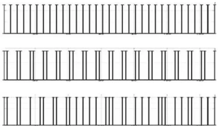
Example 1.1.1: Hidden non-linearity and the level of the input signal/1.
Fig. 1.1.1 The system under study is composed from a 3rd order Butterworth high-pass filter (input linear system), a static nonlinearity: y t( )=u t( ) .05+ u t2( ) .1+ u t3( ) .025+ u t4( ) .01+ u t5( ) and a 3rd order Butterworth low-pass filter (output linear system), connected acc. to the Wiener-Hammerstein block-structure (see Section 2.4). The Empirical Transfer Function Estimate (ETFE, [125]) of this system is measured from a single application of the harmonic excitation (odd random phase multisine, see Section 3.3) containing 409 frequency
2 With the increasing number of the measurement data the linear (and time invariant) identification techniques always provide an unfalsified linear model with the uncertainty decreasing to 0, regardless of what is the true nature of the measured system. The reason lies in the fact that the linear techniques use only second order signal statistics and that they cannot make distinction between the system and its second order (least squares) linear approximation [127].
components with uniform amplitudes, under noiseless measurement conditions. The power level of the excitation was adjusted (from left to right) as σ = 0.01, 0.1, 0.5, and 1. For small input levels the behavior of the system is convincingly linear, but for higher input levels the nonlinearity steps in more forcibly producing a seemingly random "noisy behaviour". An inexperienced user is here potentially at risk of misinterpreting this phenomenon from the linear theory point of view. Please note that an odd multisine excites only odd harmonics, i.e. the last of the 409 harmonics falls on the 818th frequency index. All the subfigures but the last to the right are printed overlapped for better visual comparison.
General note on the figures in the dissertation
The majority of the presented results are analytic and the figures serve only the purpose of illustration. Figures are based on discrete system Matlab(R2007b) simulations, using usually Wiener-Hammerstein system structure with various input and output linear systems, and polynomial static nonlinearities. The frequency band [1 … fmax] to excite the nonlinear system is always chosen to ensure that dmax * fmax < fs/2, where dmax is the maximum order of the nonlinearity and fs is the sampling frequency. The frequency axis of the figures usually shows the harmonic (frequency) index, and in some cases the relative frequency (as used in the parametrization of the Matlab functions).
Example 1.1.2: Hidden non-linearity and the level of the input signal/2.
A seemingly linear system y(t)=u(t)+εu3(t), ε=.01 is measured in the noiseless measurement setup and is modeled as yM(t)=αu(t). Its Empirical Transfer Function Estimate (ETFE) α is measured with zero mean Gaussian signal u(t) of σ =1 as α=E y t u t{ ( ) ( )} / {E u t2( )} 1 3= + ε σ2=1.03. In the truly linear ε=0 noiseless case the MSE = E{(y(t)−yM(t))2} would be zero. Now the MSE = 6ε2σ6= 0.0006, which can be easily mistaken for some residual noise. The fraction of the non-linear power in the output seems also negligible:
% 14 . 0 ) 15 6
/(
15
% 100 )}
( { / } )) ( {(
%
100 E εu3 t 2 E y2 t = ε2σ6 σ2+ εσ4+ ε2σ6 = , (1.1.1) and we may be satisfied with the linear identification results. In different experimental conditions, such model can be a source of trouble. Assume that the input is amplified 4 times (σ = 4). The fraction of the non-linear power is now 16.4%, and the MSE is 2.457 clearly indicating that the linear model is not serving its purpose.
Linear system theory is well developed and used efficiently, even if one may suspect or know that in the reality the system violates linearity assumptions. Linear system theory offers numerous advantages, like canonical model structures and the full theoretical equivalence between the identification problem posed in the time or the frequency domain, or as the input- output and the state-space models. In the following thus we keep on the linear measurement techniques we are however aware that we measure nonlinear systems. A typical situation will be where the non-linear part is negligible within the actual experimental conditions, the nonlinear behaviour contributes little to the measurement results and can be considered a kind of (nonlinear) distortion, but it will be in the interest to the user to know how serious such a distortion could be.
The state-of-the-art non-linear system identification, delivering a model describing well also the distortions, would of course yield answer to every question ([198, 188, 19, 104, 89-91, 54, 155]). In many cases it will be yet impractical at least for two reasons. First, the non-linearity is usually responsible for only a small fraction of the phenomenon, so why to pay the full cost of the parametric non-linear system identification? Second, we do not really want to know the
model of the non-linear distortion exactly, but only its influence on the originally identified linear model.
The literature shows that there is a considerable demand to embedd the nonlinear measurements in the linear measurement techniques, as this approach addresses a realistic situation. It also opens up possibilities for easier and faster measurements in the applications where the investigated system or behaviour is inherently nonlinear, but nobody wants or has the experience to tackle it with fully developed nonlinear models.
In the following we seek answers to these problems. We propose solution to the situation where the system under study shows non-linear behaviour and we show how to express its influence as errors to the measured linear Frequency Response Function (FRF), sidestepping thus the full parametric non-linear system identification. In designing the methods we keep in mind that the computing time is cheap, but the experiments are expensive (duration, or if sophisticated measurements are needed). The ideal solution would be to amend the linear FRF measurements in such a way, that the non-linear effects can be measured, or at least qualified in parallel with the main linear experiments, without extensive additional measurements or nonlinearity tests.
1.2 Overview of the literature
Modeling nonlinear distortions to linear systems (i.e. modeling weakly nonlinear systems) is a widely research field with continuous influx of the new theoretical and practical contributions.
Linear approximation to the nonlinear behavior became very early the focus of interest. In the context of control [6] used Booton’s decomposition of a static non-linearity into the best fitted (in the mean square sense) linear part and a “distortion factor” to analyze control systems with random inputs. J.L. Douce investigated the effect of the static non-linear distortions and their spectral behavior under random excitations [51, 53]; he even proposed a random-signal generator based upon the harmonic intermodulation due to non-linearity [52]. Distorting effect of the non-linearity on the input spectrum was analyzed in [263], and an interesting analysis of the static non-linear MIMO systems based on the separable signals was published in [264].
Probably the first serious attempt to deal with the non-linear distortions as a separate object of investigation, yet still within the linear system identification setting was [65]. Static or Volterra-like non-linear distortions of low order were tackled there from the measurement point of view, under harmonic excitations, within the deterministic setting. His aim was not to describe the non-linear distortions in general, but to get rid of them in concrete measurement and identification situations. To this purpose various kinds of harmonic signals were introduced [66-69], then a special kind of multisine signals was developed, to minimize the non-linear distortions for the assumed particular order of the non-linearity [70]. Later the investigations were extended to the concept of the best linear approximation to a Volterra system excited by the multisines with random harmonics (amplitudes and phases, or only phases), proposed by [30*]. Using Crest Factor minimization introduced in [85] in a series of
papers [72-73], [219-221, 223-225] presented heuristic comparison of modeling nonlinear errors if the Crest Factor minimization is also required.
Modeling non-linear systems with so-called output-error linear time-invariant second order equivalents (OE-LTI-SOE), within the Gaussian and the quasi-stationary framework, was introduced in [55-58], [125-127]. The analysis focused on the Non-linear Finite Impulse Response (NFIR) systems and the full characterization of stable causal OE-LTI-SOEs of such systems was given in [59-61]. The problem of the non-linear distortions was addressed via the notion of slightly non-linear system [58]. Seeking general conditions for the SOE of an NFIR system to be also a FIR system, separable signals were used as an extension to the notion of Gaussianity [59]3. Bounds on the distance between the SOE and the linear part of the non- linear system were also studied.
Theoretically the most rigorous setting was the approach of Mäkilä and Partington, with the deterministic framework based upon the notion of the Generalized Harmonic Analysis (GHA) and quasi-stationary signals, drawing upon the normed space operator theory. In [134] the Frechet derivative was used to derive the best causal linear approximation of mildly non- linear systems. Beside the mean square error approximation, the absolute error approximation was also considered for smooth and non-smooth static non-linear systems in [135]. In [136- 137] distribution theory of sequences was called in to refine the results obtained earlier for GHA and quasi-stationary signals. A very interesting notion of the nearly linear system and its LTI companion was introduced in [138], with the primary aim to investigate the controllability of a non-linear (NFIR) systems through the control of their LTI companions4. This work was extended in [139] to the linear approximations with the FIR and ARX parametrization, then in [140] to the notion of a non-linear companion system, providing also the state-space form for the linear companion.
1.3 Research focus
The reported work is based and extends the ideas put together in [27*, 28*, 30*], where the stochastic framework was proposed to deal with the Volterra-like non-linear distortions,
3 Although separable signals extend the properties of Gaussian signals with respect to the linear conditional expected value, their major disadvantage in the system identification is that the output of a linear system to a separable signal is not necessarily a separable signal. Separable signals are handy to identify systems with the non-linearity at the input (e.g. Hammerstein systems), they are not so useful where the non-linearity is hidden within the system, or at the system output (e.g. Wiener, or Wiener-Hammerstein systems) [148], [59-60].
4 Please note that the notion of a nearly linear system (and its linear companion) [138] is not comparable to the notion of a weakly non-linear Volterra series; see e.g. [15*]. The behavior of a nearly linear system, getting more and more linear as the input signal amplitude grows, does not reflect well what we observe in many practical measurement situations, where the signals are bounded, but the non-linearities (e.g. a cubic one, saturation, dead- zone) are not asymptotically linear. For small signals, the linear companion of such non-linear linear system can still yield large approximation errors, the related linear dynamic system of a weakly non-linear Volterra series, on the other hand, will always be closed to its linear component [162], [15*].
randomizing them through the randomization of the input signals, for which, due to the practical measurement reasons, random multisine excitations were used.
Contrary to the other contemporary approaches the aim was not only to produce the “best”
linear approximation to a weakly5 non-linear system, but to observe (and to influence) where and how the non-linear distortions manifest themselves in the measured linear non-parametric Frequency Response Function (FRF) (i.e. Empirical Transform Function Estimate – ETFE [125]). The theory was developed for input signals with a finite number of harmonics, and the asymptotic properties have been analysed when the number of harmonics tends to infinity6. The stochastic setting was essential to our purpose; otherwise there would be no possibility to qualify the error on the approximation. The stochastic setting makes it possible to design measurement procedures (here it was averaging) warranting the proper approximation of the theoretical limiting results (expected values) from the finite measurement data.7
Harmonic random signals are in the limit (in the number of harmonics) normally distributed, and even separable, the measured ETFE tends thus asymptotically to the FRF of the OE-LTI- SOE of a non-linear system described by a convergent Volterra series. Issues like stability, causality, memory length, impulse response structure, etc. are no investigated for the non- parametric FRF. However they may be pertinent to the parametric identification, which can be made after the analysis of the measured non-parametric FRF yields hints w.r.t. to the dynamics.
It is important to observe that the measurement of the non-parametric FRF precedes always, as the necessary introductory step, the parametric modeling in the frequency domain. The accurate judgement of the linear properties of the identified system, but also of the possible non-linear errors is essential for the successful further identification. The proposed methods
5 There are many definitions of being weakly non-linear or almost-linear (e.g. based on the coherent and incoherent output power, ratio of norms, ratio of coefficients, etc.), all sharing the notion that while nonlinear effects are essential and are observable, the linear behaviour dominates, and as a first approximation, the system can be considered linear.
6 Historically the starting point was the adoption in the 1980s by the Vrije Universiteit Brussel ELEC (Fundamental Electricity and Instrumentation) Department of the frequency-domain identification of the linear systems (contrary to the dominating then time-domain) and the following intensive research for the suitable deterministic excitation signals. From that time stems e.g. still state-of-the-art crest factor minimization technique [85]. Making research at the ELEC in the knowledge intensive signal processing methods ([24*-26*, 1*-*4*]) I joined the group which started to tackle the non-linear problems and became a member of the team working out the basic theory [27*-28*, 30*]. During multiple visiting periods at the ELEC I dealt with a number of open SISO (Single-Input Single-Output) problems and later I worked out the respective MIMO (Multi-Input Multi-Output) theory and solved some other open problems. From that time on this theory is intensively researched by a number of scientific and application groups.
7 Stochastic setting resembles the so called stochastic embedding of [129-130]. Stochastic embedding is a parametric framework where modeling errors are considered realizations of a random variable with a parametric distribution and the effort is to estimate these parameters. Our approach is nonparametric and the modeling errors will be classified into (nonparametric) systematic deterministic and stochastic components.
make it possible to measure the non-parametric FRF and to qualify the non-linear errors within the same experiments, minimizing the required measurement time8.
In the following I review the principal assumptions underlying the research, and the basic theoretical concepts and results. Then I present my own research results, and finally I give a summary of the impact of these results on the applications.
Basic equations of the Volterra series in the time and the frequency domain under harmonics excitations can be found in [34, 198, 22, 9, 112]. The more specific results are referenced locally.
1.4 Research assumptions
The field of non-linear systems is too vast and too complicated to tackle with success any particular problem without carefully devised limiting assumptions. Their role is to bring the problem to the size and scope still valuable in practical modeling situations, yet admitting theoretical analysis and synthesis. The essential working assumptions were applied thus to the selection of the:
• non-linear system class,
• excitation signals,
• focus of the research.
The focus is the measurement methodology of the nonparametric linear frequency characteristics (Frequency Response Function - FRF), via its Empirical Transfer Function Estimate (ETFE [125]). Due to this reason the results were formulated in the frequency- domain for the input-output system descriptions. The information available in the time- domain and in the frequency-domain measurements is the same and the formulation of the measurement problem is in itself equivalent. Nevertheless the required information appears differently in the measurement data paving the way to the advantages stemming from different processing algorithms.
To the advantages of the frequency-domain belong the freedom in the selection of the frequencies where the model is matched to the measurements or freedom in restricting unwanted frequences, the possibility to model unstable systems, furthermore, if abiding to the periodic excitations (and periodic reference signals), no leakage bias on the ETFE, separation of the plant and the output noise modeling, possibility for the nonparametric noise modeling, possibility for modeling under close-loop conditions, finally (what is the topic of this work) the separation of the effect of the non-linearities and the output noise [204, 206, 125].
8 In recent developments the originally proposed harmonic random excitations are perturbed (power level, coloring) to verify how does it perturb the measured linear ETFE to gain indication about the possible structure of the nonlinear block model [63-64, 212-213, 114-116].
.
The non-linear system theory, as mentioned before, suffers from the multitude of possible models. Furthermore, the non-linear system identification is conditioned on the used excitation signals due to the presence of unavoidable model errors. Even if we intend to tackle practical situations when the level of the non-linear distortions is low, the choice of the class of the non-linear system models and the associated choice of the input signal class is important, as it is heavy in the consequences.
On the system and signal models
In the present work convergent Volterra series were assumed as the model the measured systems. The particular usefulness of such model is dictated by the following (summarizing the wisdom of [23-25, 19, 21-22, 202, 211, 54, 59-60, 104, 137, 134, 162, 198, 188, 76]):
1. Natural (additive) way of how the linear and non-linear systems can be treated together, and the level of the non-linearity controlled;
2. A number of pragmatically important non-linear systems can be already modeled by finite, low order Volterra series;
3. Wide class of (even non-continuous) non-linear systems which can be approximated in the least square sense with the Volterra series;
4. Well developed frequency-domain representation;
5. Natural way of how the non-linear dynamics can be modeled;
6. Volterra models contain a number of practically important non-linear block models, i.e.
Wiener-, Hammerstein-, and Wiener-Hammerstein models; and also Non-Linear Finite Response (NFIR) models;
7. Straightforward extension of the Single-Input Single-Output (SISO) models to the Multiple-Input Multiple-Output (MIMO) models;
8. Possibility to include a priori physical knowledge into the models (the number, the order, the symmetry, and the frequency bands of the Volterra kernels);
9. Volterra-series possess a unique steady state property and are Periodic-Input Same Periodic-Output (PISPO) systems, i.e. they do not generate subharmonics. Volterra series also yield almost periodic outputs to the almost periodic excitations.
Volterra models are not a universal tool and their expressiveness is limited. A number of interesting and important non-linear phenomena cannot be modeled well or at all with the Volterra series. As the Volterra series generalize the Taylor expansion, bifurcations, chaos, non-linear resonances, generation of sub-harmonics, etc. are out of reach for the Volterra models.
The second principal choice applied to the input excitation signals. Asymptotically Gaussian periodic signals were adopted (over non-periodic signals) due to:
1. Less problems in the ETFE measurements (no leakage due to transients);
2. It is easy to distinguish or to separate the input signal properties (periodic) from the noise properties (non-periodic);
3. An easy introduction of the randomness into the signal (via random phases and/or random spectral amplitudes);
4. A free hand in the construction of different signal characteristics by manipulating the spectral properties (coloring), the frequency grid, and the phases;
5. An easy realization of such signals in modern signal generators, meaning that the developed theory is straightforward enough to be widely used in practice;
6. Possibility to model approximately the non-periodic signals also by choosing high enough number of the harmonics in a bounded frequency band.
7. Considering that in many measurement application areas Gaussian (noise) signals are traditionally used, the proposed excitations signals provide portability of the new methods combined with additional advantages;
8. Gaussian signals are "non-linearity-friendly" (i.e. when applied to static non-linear systems).
9. Last, but not least harmonic signals can be analytically integrated and/or differentiated sparing error prone signal processing where different forms of the excitations are jointly needed (e.g. velocity, angular position, acceleration [227]).
It is important to mention, that the approach presented in the following and based on the characterization of the non-linear distortions as a noise and bias on the linear FRF, is valid for any convergent Volterra series, i.e. for any smooth enough non-linear dynamic system. If however the non-linear behaviour is strong, using such linear model does not make sense, as the excessive non-linear noise will make the measurements long and costly and then still the bias to the linear FRF will be too large to get a feeling of what the linear system dynamics is really like. Despite hence the universal validity of the results, their practical usage is confined to the situations where the level of non-linearity is small and/or the order of the non-linear system is low.
Research methodology
The aim of the research was to separate in the measured FRF of a weakly non-linear system the systematic non-linear effects (resident and enduring in the measurement results) from other, noise-like non-linear effects that are removable with a suitable post-processing.
To this end it is not enough to excite the system (like a linear system) with a single deterministic signal. A manageable stochastic process is needed, to excite the system with its sample functions, one after the other. The non-linear system will answer to every input sample function differently, camouflaging the systematic error (with respect to the linear system) with
"non-linear noise" of varying behavior (see Example 1.1.1).
Considering that the input to the investigated system is a stochastic process, the system output will be a stochastic process alike and in principle the systematic (non-zero expected value) and "noise-like" (zero expected value) error components can be grasped by computing higher order moments. Higher order moment estimates can be computed by assembly averages. In the measurement technical language it means that we should generate independent sample functions from the input stochastic process, apply them as excitations to the system, and then average the individual measurement results.
The used (usual) sample mean is appropriate because (1) sample averaging is a consistent estimate of the theoretical expected value. The practical bound limiting the number of averages is only the measurement duration (cost of the equipment, not met stationarity conditions, etc.); (2) for Gaussian signals the average is also a minimum variance estimate;
(3) an average can be computed recursively without unnecessary data storage (important due to (1))9.
At the beginning of the research the used excitation signal was the periodic Gauss noise (so called periodic noise). The break-through was however brought by the observation that if the phases of the multi-harmonic signals are random, independent, and uniformly distributed on the unit circle, then with the increasing number of the harmonics such signal - called random multisine - tends to a Gaussian signal. Furthermore the FRF measurements performed with random multisines tend asymptotically to the measurements performed with Gaussian signals, also in case of the non-linear systems.
1.5 Summary of the scientific results
The basic concepts of the underlying theory were established at the VUB ELEC Department, but due to the frequent research visits (from University of Glamorgan (UK), University of Warwick (UK), Linköping University (S), KTH Royal Institute of Technology (S), and last but not least the BME researchers) the developments were discussed continuously almost on the daily basis and were published in deliberately jointly authored publications (at the Department of Measurement and Information Systems, BME, these contacts took between 1997-2006 the organizational form of 4 successfully concluded Hungarian-Flemish Bilateral Research Grants).
Among the scientific results there are thus results, especially from the beginning of the years long research, where the identification of the individual responsibility of the authors is not possible, but there are also results, which I can responsibly call my own, despite the joint authorship of the publications. Such inseparable results merit mentioning because they reveal the research process and provide the context for presenting the strictly individual contributions. After summary review of the joint results, the individual contributions are structures into the research Theses, to make a clear distinction in the presentation.
9 In recent developments, due to the industrial technological demands, discrete level excitation signals were also considered leading to the “nonlinear noise” of different properties where the processing of the measured results was based on median filtering instead of simple averaging [210, 268-269].
Jointly achieved research results
The starting point was the development of the theory of the nonparametric best linear approximation to weakly non-linear SISO (Single-Input Single-Output) systems. We gave the mathematical structure of the approximation and established the theoretical and practically verifiable properties of its components. This theoretical approach was extended, supported by analysis, simulations, and practical suggestions, to the measurement technology of the linear frequency characteristics ([27*-28*, 30*-31*, 33*-37*, 40*, 42*, 45*]). (Sections 2.2-2.3-2.4) One of the important design parameters in the measurement technology was the frequency grid of the multisine excitations, frequencies where the excitation injects energy into the measured system. The selection of the frequency grid in the non-linear measurements strongly influences the properties of the measurable quantities. In our research many kinds of grids were considered pursuing inherent theoretical and practical possibilities ([32*, 247, 162, 170]) (Sections 3.2-3.3)
Expected values measured on the Volterra series with the harmonic signals with a large number of harmonics theoretically correspond to the Riemann integral sums. This made it possible to evaluate theoretically the robustness of the asymptotic properties of the systematic error (Best Linear Approximation - BLA) measurements. [17*]. (First part of Section 3.6) An interesting and pragmatically important issue was the fact that in the designed (Best Linear Approximation) measurements the non-linear noise variance is directly measurable, but not so the non-linear bias (i.e. the systematic error on the FRF). Research attempted to clarify how much these two error components are interdependent, with the prospect to estimate the systematic FRF error from the measurements of the nonlinear noise variance.
[47*-48*]. (Section 2.5, equ. 2.5.14)
Finally if the non-linearity is weak, linear system analysis may perhaps indicate that there are no problems with the stability in the close loop. The amplitude of the signals in the feed-back loop may nevertheless increase so much that the non-linear effects will appear with potentially unfavorable consequences. Some research was done to predict such situation well in advance ([38*, 41*, 43*]). (Section 6.3)
Contributions to the SISO theory
The strictly joined research not only established the basic theory but also led to the formulation of a vast number of problems (not everyone solved yet) where the scientific contributions can be already attributed to the concrete individuals. In case of SISO systems, I have dealt in particular with various aspects of the multisine design and the systematic nonlinear error in more specific measurement situations. These particular research problems and results are formulated as independent research Theses.
Thesis Group 1. Design methodology of multisine excitation signals – SISO systems Here I have collected results where the topic of the research was the flexibility of the multisine signals, shaping them to the application requirements and then analysing the related problem of how similar are the measurement results if the excitation signals differ in the design.
Problem Topic 1.1 Before the theoretical and the practical well-founding of the multisine signals with a large number of harmonics the prevalent excitation signal in a number of measurement fields was the Gaussian noise. In theory both signals are asymptotically equivalent, but for the credibility the non-asymptotic behavior of the multisines had also to be examined.
Thesis 1.1. Design considerations how to chose multisine excitation signals
Based on the investigation I have proposed a methodology how to use multisine signals if nonasymptotic behavior is also important. In measuring the FRF of a weakly nonlinear systems I propose to use odd-odd (double odd: every second odd harmonic frequency) random phase multisine considering that:
- the measured FRF is the same as measured on the system with the Gaussian signal,
- the uncertainty of the measurement is largely reduced due to the drop-out of the effects of the even and in part of the odd nonlinearities (see Fig 3.5.1),
- it is possible to separately measure the even and odd nonlinearities.
It can be also stated that in case of the Gaussian noise excitation the required frequency band limitation and the amplitude censoring amplify the bias on the measured FRF, if the measured system does contain odd nonlinearities. Furthermore the usual amplitude censoring by ± 3 σ is not enough if the nonlinearity is involved (I propose censoring by ± 4 σ). [49*-50*, 5*, 8*, 12*, 39*]. (Sections 3.2, 3.5, Th 3.2.1)
Problem Topic 1.2 Frequency grid is the design parameter of the multisine signals.
Frequency grids of various structures can be successfully used to solve special measurement problems. Important question is how consistent could be the measured FRF Best Linear Approximations, if the used multisine signals differ in the definition of the frequency grid?
Thesis 1.2. Unifying asymptotic results for different frequency grids of the multisine excitation with the theory of the uniformly distributed sequences
I have determined that if the frequency grids are are modeled as the uniformly distributed sequences with increasing resolution, then the error between the measurements obtained from different frequency grids gets smaller and is of the order of the magnitude of the grid resolution [20*, 46*]. (Section 3.6, from Def 3.6.1, Th 3.6.2)
Problem Topic 1.3 In measuring non-linear systems an important issue is the control of the amplitude density of the excitation signals. It is a tool to put signal energy at the amplitudes relevant for the nonlinear behavior.
Thesis 1.3. Designing application dependent wide band multisine excitation signals I have determined that the phases of the multisine, which are a design parameter, with suitable phase iterating algorithms, can be used to the user-demanded forming of the amplitude density of the multisine signal. Moreover, with some trade-off, the crest factor minimization can be also included [29*]. (Section 3.4, Algorithms 3.4.1-3.4.3)
Thesis Group 2. Properties of the systematic nonlinear errors – SISO systems
Here I have collected results of investigating in more detail the properties of the systematic error component and the mutual relation of the systematic and the stochastic nonlinear errors.
Problem Topic 2.1 The systematic error on the FRF Best Linear Approximation measured in the presence of the non-linearity is in itself not measurable, however the variance of the non- linear noise is measurable. Important problem is to find out how the measurable (stochastic) error can be used to estimate the nonmeasurable (systematic) error.
Thesis 2.1. Establishing bounds on the systematic error of the Best Linear Approximation
I have determined that for the static polynomial non-linearity the cubic system can be considered the worst case instance and based on it I have formulated the worst-case estimate of the non-measurable error. I have extended the estimate heuristically to the Wiener- Hammerstein system model [9*]. (Section 2.5, Ths 2.5.3-2.5.4)
Problem Topic 2.2 The coherence function is a well known tool in the recognition and examination of the non-linear systems (considered as black-box models). If the non-linear system admits the non-linear additive noise model, how this additional knowledge will influence the behavior of the coherence function?
Thesis 2.2. Clarification of the relation of the Best Linear Approximation and the coherence function
I have established that the coherence function can be expressed with the components of the Best Linear Approximation (non-linear bias and noise), as well as that the nonlinearity indicating properties of the measured coherence function are consistent with the behavior of the components of the Best Linear Approximation. To this end I have investigated general and also more specific non-linear system structures [10*-11*]. (Section 2.5, Ths 2.5.1-2.5.2) Problem Topic 2.3 The researched question was whether the product of the Best Linear Approximations to the superposed non-linear systems can be used to build an acceptable approximation of the whole system.
Thesis 2.3. Analysis of the superposition of the SISO systems from the point of view of the Best Linear Approximation
I have determined that in the frequency domain where both system components show high coherence, the product relation of the linear system theory (i.e. that the frequency
characteristic of the superposition is the product of the frequency characteristics of its components) remains valid [10*-11*]. (Section 6.1)
Problem Topic 2.4 The Best Linear Approximation FRF is traditionally measured as a sample mean (for linear systems the minimum variance Maximum Likelihood estimate for Gaussian excitations). This minimum variance is the basis of the usual measurement time vs.
measurement quality trade-off. However due to the non-linearity the sample mean is no more an optimal estimate; its variance is not an attainable theoretical minimum and can be improved. By using a limited a priori knowledge about the measured system this trade-off can be made sharper.
Thesis 2.4. Reducing the measurement time of the Best Linear Approximation by Monte Carlo averaging methods
I have developed an alternative method of measuring the Best Linear Approximation where a better trade-off between the measurement duration and the measurement accuracy can be achieved by using the Monte Carlo variance reduction techniques, without increasing the complexity of the measurement protocol [23*]. (Section 6.4)
Contributions to the MIMO theory
In the real life problems there are usually more independent effects cumulated towards a common output. It is important thus to handle Multiple-Input (Multiple-Output) models also.
It is also expected that the earlier SISO case should appear as a special case within the MIMO theory.
Thesis Group 3. Properties of the systematic nonlinear errors – MISO systems
Based on SISO Best Linear Approximation theory I have developed the ground results in the MIMO (MISO) Best Linear Approximation theory, focusing on the description of the systematic errors and the equivalence of the measurements for different kinds of excitations. I also have extended to the MISO case some of the more specific results developed for the SISO systems.
Problem Topic 3.1 In case of multiple input systems separate Best Linear Approximations can be defined for every input-output signal channel. In computing such BLA system other inputs act as disturbances and complicate the computation of the non-zero expected values.
Similarily to the SISO case some kernels do not contribute to the systematic errors, however the general picture is much more complicated.
Thesis 3.1. Developing general MIMO BLA theory from the point of view of the systematic FRF error
I have determined that using the random multisine BLA SISO measurement technique, the 2- dim MISO cubic system excited with independent random multisines defined on a common frequency grid, can be modeled (similarly to the SISO case) as a 2-dim linear FRF
characteristics and the nonlinear output noise [22*, 13*-14*, 44*]. (Sections 4.1-4.2, Ths 4.1.2, 4.1.3, 4.1.4, 4.1.5). As a full generalization I have determined that the multiple-input Volterra system excited with the random multisine excitations can be expressed as a linear BLA FRF system network, completed with the output non-linear noises. The earlier SISO and 2-dim results are the special cases of the general case [15*, 20*] (Sections 4.5-4.6, Ths 4.5.1, 4.5.2, 4.6.1)
Problem Topic 3.2 Similarly to the SISO systems (see Thesis 2.3) an interesting question for the MIMO systems is how robust is the FRF BLA matrix from the point of view of further distortions superposed on the system.
Thesis 3.2. Superposition of the MIMO systems from the point of view of the Best Linear Approximation
I have established that the Best Linear Approximation to a MIMO system is robust when the excitations are nonideal and are modelled by the output of a nonlinear Volterra MIMO system.
I have established that the nonlinear distorting effects cause larger FRF characteristics errors than the linear distorting effects of similar amplitude, the distorting effects originated in the cross input-output signal paths cause larger errors than the distorting effects in direct signal paths, as well as that the FRF phase errors increase faster than the FRF amplitude errors.
[18*] (Section 6.2)
Thesis Group 4. Design considerations about the excitation signals – MISO systems Multiple inputs introduce additional freedom into the excitation design. Not only we dispose the design parameters at a single channel, we can also decide how the excitations at different input channels and in different experiments could be related to yield better measurement results. The challenge lies in designing excitations that are better from the measurement technical point of view (i.e. warranting equivalent measurements at a lower cost). In case of multiple inputs a distinction must be made between the 2-dimensional and more-dimensional weakly nonlinear systems. Surprisingly, in low nonlinear order 2-dimensional system measurements the traditional (linear system theory) noise attenuating techniques are henceforward applicable, but this advantage is lost for higher order nonlinearity and/or higher input dimensions. There new noise attenuation techniques has to be developed.
Problem Topic 4.1 In linear MIMO measurements an important part of the measurement methodology is the input design suitable for the noise cancellation. I have investigated whether such noise cancelling methods could be also used to the advantage in the BLA measurements to cancel the non-linear noise.
Thesis 4.1. Optimizing excitations used in the 2-dim BLA theory
I have determined that the linear noise attenuating technique is in the same way effective in case of the 2-dim cubic BLA measurements. I have also determined that this approach is not suitable in case of the system of a higher nonlinear order or the higher number of the inputs.
[22*, 13*-14*, 44*] (Sections 4.3, 4.4)
Problem Topic 4.2 The MIMO extension to the SISO BLA theory was formulated for the random multisine signals. An important question however is whether the excitation signals asymptotically equivalent in the SISO theory (multisine, periodic noise, Gaussian noise) are similarly equivalent in the MIMO case.
Thesis 4.2. Equivalence of the excitations from the point of view of the systematic (MIMO) FRF error
I have determined that the Gauss noise, the periodic noise, and the random phase multisine signal classes are asymptotically equivalent (if the number of harmonics is increasing and the spectral properties of the signals are comparable) also in the case of nonlinear MIMO Volterra systems in a sense that using these excitation signals the measured multidimensional FRF BLA systems tend in the limit to the same transfer characteristics matrix. [21*] (Section 5.4, Ths 5.4.1, 5.4.2)
Problem Topic 4.3 In the detailed presentation of the results referred in Thesis 2.4 one can see that in the multidimensional case the inverse of the input matrix amplifies uncertainty, even in case of the multisine excitations (contrary to the SISO case). An important question is whether this situation can be improved or not?
Thesis 4.3. Special orthogonal random multisines
With the introduction of orthogonal random multisines I have developed a new efficient method of measuring the Best Linear Approximation of the MIMO Volterra systems. I have proved that the newly introduced excitation signals are equivalent in the sense of the Thesis 2.4 to other listed excitation signals, but result in an essentially lower level of the non-linear noise experienced on the measured FRF characteristics. [15*-17*] (Sections 5.1-5.2, Ths 5.1.1, 5.2.2, Lemma 5.2.1)
1.6 Review of the content
Section 2 introduces the general theory for the single-input single-output (SISO) systems.
First a simple example is shown, without the in-depth formalism, providing the feeling of the problem and yet presenting every important issue and question, which later on will be elaborated in detail (Section 2.1). Section 2.2 presents the main result, i.e. the additive non- linear noise model to the non-linear system, and then the properties of the systematic non- linear distortion (Section 2.3) and the stochastic non-linear distortion (Section 2.4) are analyzed. As mentioned before, the Volterra models cover the usual non-linear block models.
The developed theory is applied to them in Section 2.5. Finally the question of the mutual analysis of the distorting bias and variance is considered in Section 2.6.
The purpose of Section 3 is to show the enormous flexibility of the multisines as the excitation signals. Section 3.1 discusses tunable free parameters, i.e. the frequency grid, the amplitude spectrum, and the phases. Then various types of the multisines are presented (Section 3.2), discussing their design and the intended effects on the measured linear
approximation. The aim of Section 3.3 is to show, that the measurement results obtainable with the multisines are comparable for the increasing number of harmonics with the results obtained with traditional excitation signals (Gaussian noise and periodic noise).
Section 4 extends the results of Sect 2. to the multiple-input multiple-output (MIMO) Volterra models. The main result, the multidimensional additive non-linear noise model, is developed in Section 4.1 and the properties of the non-linear biases and non-linear noise variances are evaluated in Section 4.2 and 4.3.
In MIMO measurements excitations are applied to more than one input simultaneously. The excitation signals must be designed thus not only in themselves, but also in relation to the signals applied at other input points. Section 5 presents excitation design problem for the MIMO systems. Free design parameters are discussed in Section 5.1. Various excitation schemes and their effect on the model developed in Section 4 are analyzed in Section 5.2.
Finally in a manner similar to Section 3.3 the equivalence of the measured results for various MIMO excitation schemes is considered.
Section 6 presents some applications of the introduced theory. In Section 6.1 simple measurement application are shown, based on the literature. Sections 6.2 and 6.3 elaborate on the problem of non-linear distortions in cascaded systems, for SISO and for MIMO systems respectively. Besides modeling practical measurement problems cascaded systems make it possible to study the robustness of the developed theoretical tools. In Section 6.4 an attempt is made to qualify stability problems in the non-linear feedback system based on the additive non-linear noise model.
In the development of the additive non-linear noise model, necessarily, plenty of problems remain still open. Section 7 discusses some of the more interesting and difficult open research issues.
Finally the Appendices contain the most lengthy proofs and examples.
2. General SISO theory
An unexpected non-linearity can deceive the user not familiar with the non-linear phenomena, or the user versed solely in the linear measurement or identification methods, making her/him thinking that the nature of the problem is quite different. Consider simulated measurements in the Example 1.1.2. The FRF of a linear system, otherwise smooth, can become scattered and acquires the “noisy look” if the excitation signal hits the hidden non-linear component.
Besides scattering, the measured FRF will also be biased, this though is more difficult to discern, as the true frequency dependence of the characteristic is not known in advance. It is common knowledge, however, that without the noise, the FRF measurements should yield more or less smooth functions. The visible “noisiness” can thus easily be taken as the proof that the output noise is the real problem here (especially as it is usually present). The scattering is caused by the non-linear mechanism of summing various harmonic components in the input signal and shifting them to different places (frequencies) along the frequency axis.
Example 2.1: Scattering of the frequencies due to a non-linearity. Let the system y(t)=u(t)+εu3(t) be excited by the input signal containing two harmonic components with frequencies ω 1 = 1 and ω 2 = 4. Then the output signal will have harmonics at frequencies ±1, ±2, ±3, ±4, ±6, ±7, ±9, ±12.
2.1 Problem introduction via simplified examples
In this Section the main points of the theory developed formally later will be shown in simplified measurement examples, without strict definitions and derivation.
A. Measuring a linear system with a random signal. Assume that for linear FRF measurements a periodic random u(t)=u(t,ξ) stochastic process input signal is used. Let the collected measurement data come from noisy linear system, where the zero mean output noise is similarly a stochastic process bound to a random event ζ, then:
) , ( ) , ( ) ( )
(t G0 q u t ξ n t ζ
y = + , or (2.1.1)
in the frequency domain (l is the discrete frequency)10: Y(l)=G0(l)U(l,ξ)+N(l,ζ). (2.1.2) The FRF is computed (from k = 1… M experiments) as:
∑
∑
∑
∑
= +=
k k M
k k k M
k k M
k k k M
l U
l U l l N
G l
U
l U l l Y
G 1 ( ) 2
) ) (
1 ( 2 0
) 1 (
) ) (
1 (
| ) , (
|
) , ( ) , ) (
(
| ) , (
|
) , ) (
ˆ(
ξ ξ ζ
ξ ξ )
(
(2.1.3)
This estimate is unbiased, i.e.: E{Gˆ(l)}=G0(l), (2.1.4) because the output noise and the excitation are independent:
10 Considering that Y is the output to the stochastic input and contains also random noise, formally we should write: Y(l) = Y(l, ξ, ζ) and similarly G(l) = G(l, ξ, ζ), however these arguments have been omitted for clarity.
0 }
| ) , ( {|
)}
, ( { )}
, ( } {
| ) , (
|
) , ( ) ,
{ ( 2
) 1 (
) ) (
1 ( ) 2
1 (
) ) (
1 (
=
=
∑
∑
∑
∑
k
k M
k
k k M
k k M
k k k M
l U E
l U E l N E l
U
l U l E N
ξ
ξ ζ
ξ ξ ζ
ξ
ξ ζ
ξζ . (2.1.5)
and its variance depends on the degree of averaging introduced in (2.1.3).
Note: For the random multisine signals considered later: Eξ{U(l,ξ)U(l,ξ)}=Uˆ2.
B. Measuring a non-linearly distorted system with a deterministic signal. To measure the linear FRF it is enough to keep a single input realization (i.e. let ξ = ξ0) and to average the results to get rid of the output noise N(l,ζ). Reassured that we can thus simplify the measurement we continue overlooking the point, that now the measurement data is coming from a noisy non-linear system:
) , ( ) , ( ) , ( ) ( )
(l G0 l U l ξ0 Y l ξ0 N l ζ
Y = + NL + , (2.1.6)
with YNL(l,ξ0)=V[U](l,ξ0) the non-linear part of the system. The FRF estimate is now:
) , (
) , ( ) , (
) , ) (
) ( , (
) , ( ) , ( ) , ( ) ( ) , ) (
ˆ(
0 0
0 0
0 0 0
0
0 ξ
ζ ξ
ξ ξ
ζ ξ
ξ
ξ U l
l N l
U l l Y
l G U
l N l
Y l
U l G l
U l l Y
G + NL + = + NL +
=
= ( )
(2.1.7) Averaging gets rid of the output noise, but the non-linear term is not random:
) , (
) , ) (
( )}
, { ( )}
ˆ( {
0 0 0
0 ξ
ξ
ξ U l
l l Y
l G U
l E Y l G
E = ( ) = + NL
, (2.1.8)
and the measurement results are heavily distorted.
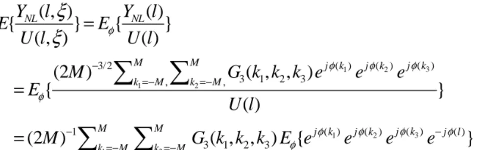
C. Measuring a non-linearly distorted system with a random signal. What will happen if we return to our original random input: Y(l)=G0(l)U(l,ξ)+YNL(l,ξ)+N(l,ζ)?
Now:
∑
∑
∑
∑
∑
∑
= + +=
k k M
k k k M
k k M
k k k NL M
k k M
k k k M
l U
l U l N l
U
l U l l Y
G l
U
l U l l Y
G 1 ( ) 2
) ) (
1 ( ) 2
1 (
) ) (
1 ( 2 0
) 1 (
) ) (
1 (
| ) , (
|
) , ( ) , (
| ) , (
|
) , ( ) , ) (
(
| ) , (
|
) , ) (
ˆ(
ξ ξ ζ
ξ ξ ξ
ξ ξ )
(
and:
}
| ) , (
|
) , ( ) , ( {
}
| ) , (
|
) , ( ) , ( {
) ( )}
ˆ(
{ 2
) 1 (
) ) (
1 ( ) 2
1 (
) ) (
1 (
0
∑
∑
∑
∑
++
=
k k M
k k k M
k k M
k k k M NL
l U
l U l N E
l U
l U l Y E
l G l G
E ξ
ξ ζ
ξ ξ ξ
ςξ ξ
ςξ .
(2.1.9) The second expected value is not a problem, as both random components are independent and zero mean. What about the non-linear expected value in the middle?
If the input signal has bounded realizations for every ξ and the non-linear system V[.] is well behaving (e.g. continuous, BIBO stable, etc.), then the output of the non-linearity YNL(l,ξ)