Polynomial differential systems with hyperbolic algebraic limit cycles
Salah Benyoucef
BLaboratory of Applied Mathematics, Department of Mathematics, Faculty of Sciences, University of Setif 1, 19000, Algeria
Received 30 March 2020, appeared 29 May 2020 Communicated by Gabriele Villari
Abstract. For a given algebraic curve of degreen, we exhibit differential systems of de- gree greater than or equal ton, by introducing functions which are solutions of certain partial differential equations. These systems admit precisely the bounded components of the curve as limit cycles.
Keywords: sixteenth problem of Hilbert, planar differential system, invariant curve, periodic solution, hyperbolic limit cycle.
2020 Mathematics Subject Classification: 34C25, 34C05, 34C07.
1 Introduction
The second part of the sixteenth problem of Hilbert still persists as a research area. It aims to find the maximum number of limit cycles of the differential system:
˙ x = dx
dt =P(x,y),
˙ y= dy
dt = Q(x,y),
(1.1)
where PandQare polynomials.
Several articles and books have been published on the analysis of the existence, number and stability of limit cycles of equation (1.1) (see for instance [5,6,8,9,15,18]).
Generally, the exact analytical expressions of limit cycles for a given differential system are unknown, except in specific cases.
This paper is a contribution in the direction of determining the number of limit cycles and giving their explicit form.
Motivated by some publications [1–4,7,11–14,16], we will exhibit polynomial vector fields, where just by choosing the components of the system satisfying certain conditions, we can conclude directly the number and the explicit form of limit cycles.
BCorresponding author. Email: saben21@yahoo.fr
2 Introductory concepts
Let us recall some useful notions.
For U∈ R[x,y], the algebraic curveU =0 is called an invariant curve of the polynomial system (1.1), if for some polynomialK ∈R[x,y], called the cofactor of the algebraic curve, we have
P(x,y)∂U
∂x +Q(x,y)∂U
∂y = KU. (2.1)
Simple analysis of equation (2.1) shows that when max(degP, degQ) = n, the degree of the cofactorKis at mostn−1 and that the curveU=0 is formed by trajectories of the system (1.1).
The curve Ω = (x,y)∈R2,U(x,y) =0 is a non-singular curve of system (1.1), if the equilibrium points of the system that satisfy
P(x,y) =0,
Q(x,y) =0 (2.2)
are not contained on the curveΩ.
A limit cycleΓ={(x(t),y(t)),t ∈[0,T]}is aT-periodic solution isolated with respect to all other possible periodic solutions of the system.
AT-periodic solutionΓis a hyperbolic limit cycle ifRT
0 div(Γ)dtis different from zero.
By using the method of characteristics to solve partial differential equations, we conclude that, the solution of equation
α∂f
∂x +β∂f
∂y =0 (2.3)
is
f(x,y) =Φ(βx−αy), (2.4)
whereα,βare nonzero reals andΦis an arbitrary function.
The solution of the equation
α∂f
∂x +β∂f
∂y =γ (2.5)
is the function f solving the equation
Ψ(βx−αy,γx−αf) =0, (2.6)
whereα,β,γare nonzero reals andΨis an arbitrary function. In the polynomial case f(x,y) = γ
αx+
∑
n k=0ck(βx−αy)k (2.7)
or
f(x,y) = γ βy+
∑
n k=0ck(βx−αy)k (2.8)
the solution of the equation
x∂f
∂x +y∂f
∂y = f (2.9)
is the function f solving the equation Ψ
x f,y
f
=0. (2.10)
In the polynomial case it can be taken as
f(x,y) =ax+by. (2.11)
Colin Christopher in his article [7] gives the following theorem.
Theorem 2.1. Let U = 0be a non-singular algebraic curve of degree m,and D a first degree polyno- mial, chosen so that the line D=0lies outside all bounded components of U =0. Choose the constants αandβso thatαDx+βDy 6=0,then the polynomial vector field of degree m,
˙
x =αU+DUy,
˙
y =βU−DUx (2.12)
has all the bounded components of U = 0as hyperbolic limit cycles. Furthermore, the vector field has no other limit cycles.
Our contribution is a generalization, which consists in introducing polynomial functions to system (2.12) and in the study of the existence of limit cycles.
3 The main result
We start by adding a polynomial function of any degree to system (2.12), which becomes,
˙
x =αU+ (ax+by+Φ(βx−αy))Uy,
˙
y=βU−(ax+by+Φ(βx−αy))Ux (3.1) and we show that system (3.1) has all the bounded components ofU =0 as hyperbolic limit cycles if the conditions of Theorem 1 of [7] are satisfied.
Theorem 3.1. Let U =0be a non-singular algebraic curve of degree m,andΦa polynomial function of degree n, chosen so that the curve ax+by+Φ(βx−αy) =0lies outside all bounded components of U =0. Choose the constants a and b so that aα+bβ6=0,then the polynomial vector field of degree m+n−1,
(x˙ = αU+ (ax+by+Φ(βx−αy))Uy,
˙
y= βU−(ax+by+Φ(βx−αy))Ux
has all the bounded components of U =0as hyperbolic limit cycles.
Proof. LetΓbe the curve ofU=0.
Note thatΓis a non-singular curve of system (3.1) and the curveax+by+Φ(βx−αy) =0 lies outside all bounded components ofΓ.
To show that all the bounded components ofΓare hyperbolic limit cycles of system (3.1), we will prove that Γ is an invariant curve of the system (3.1), and RT
0 div(Γ)dt 6= 0 (see for instance Perko [17]).
i)Γis an invariant curve of the system (3.1):
dU
dt =Ux αU+ (ax+by+Φ(βx−αy))Uy
+Uy(βU−(ax+by+Φ(βx−αy))Ux)
= αUx+βUy U
where the cofactor isK(x,y) =αUx+βUy. ii)RT
0 div(Γ)dt is nonzero.
To see this, first note that Z T
0 div(Γ)dt=
Z T
0 K(x(t),y(t))dt, (3.2) see for instance Giacomini & Grau [10]. Then one has
Z T
0 K(x(t),y(t))dt=
I
Γ
αUx
−(ax+by+Φ(βx−αy))Uxdy+
I
Γ
βUy
(ax+by+Φ(βx−αy))Uydx
=
I
Γ
α
−(ax+by+Φ(βx−αy))dy+
I
Γ
β
(ax+by+Φ(βx−αy))dx.
Letω =βx−αy. By applying Green’s formula we obtain I
Γ
β
(ax+by+Φ(ω))dx−
I
Γ
α
(ax+by+Φ(ω))dy
=
Z Z
int(Γ)
∂
β (ax+by+Φ(ω))
∂y +
∂
α (ax+by+Φ(ω))
∂x
dxdy
=
Z Z
int(Γ)
−β
b+∂∂ωΦ(−α) (ax+by+Φ(ω))2 +
−α
a+∂∂ωΦ(β) (ax+by+Φ(ω))2
dxdy
=−
Z Z
int(Γ)
β
b+ ∂Φ
∂ω(−α) (ax+by+Φ(ω))2 +
α
a+ ∂Φ
∂ω(β) (ax+by+Φ(ω))2
dxdy
=−
Z Z
int(Γ)
βb+αa (ax+by+Φ(ω))2
dxdy, where int(Γ)denotes the interior ofΓ.
Asαa+βb6=0, RT
0 K(x(t),y(t))dtis nonzero.
Remark 3.2. When Φ(βx−αy) is constant, we find ourselves in the case of Cristopher’s theorem (i.e. Theorem2.1).
WhenΦ(βx−αy)is of first degree, the lineax+by+c=0 in Christopher’s theorem will be replaced by the line(a+β)x+ (b−α)y+d=0.
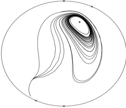
Example 3.3 (Quintic system with exactly one limit cycle). Let α = 1,β = 2,a = 1,b = 2, Φ(βx−αy) =Φ(2x−y) = (2x−y)2+1.
The system
˙
x =x4+y2−4y−3x+5+ (x+2y+ (2x−y)2+1) (2y−4),
˙
y=2x4+y2−4y−3x+5−(x+2y+ (2x−y)2+1) 4x3−3 (3.3) admits one hyperbolic limit cycle represented by the curve x4+y2−4y−3x+5 = 0. See Figure3.1.
Figure 3.1: Limit cycle of system (3.3).
Remark 3.4. Let us consider the system
˙
x =αU+f(x,y)Uy,
y˙ =βU− f(x,y)Ux, (3.4)
whereU and f areC1 functions on an open subsetVof R2. To have all the bounded compo- nents ofU=0 as limit cycles it is necessary that f satisfies the partial differential equation
α∂f
∂x+β∂f
∂y =γ, where γ6=0. (3.5)
In the polynomial case f(x,y) = γ
αx+Φ(βx−αy) or f(x,y) = γ
βy+Φ(βx−αy), which are just particular cases of Theorem3.1.
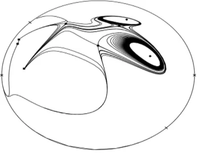
Example 3.5 (Quintic system with exactly two limit cycles). Let α = 1, β = −1, γ = 3, f(x,y) =3x+ (x+y)2.
The system
˙
x =x3−2xy2+10xy−15x+y4−10y3+35y2−50y+30 +(x+y)2+3x
4y3−30y2−4xy+10x+70y−50 , y˙ =2x3−2xy2+10xy−15x+y4−10y3+35y2−50y+30
−(x+y)2+3x
3x2−2y2+10y−15
(3.6)
admits two hyperbolic limit cycles represented by the curve x3−2xy2+10xy−15x+y4− 10y3+35y2−50y+30=0. See Figure3.2.
Figure 3.2: Limit cycles of system (3.6).
References
[1] M. Abdelkadder, Relaxation oscillator with exact limit cycles, J. Math. Anal. Appl.
218(1998), 308–312,https://doi.org/10.1006/jmaa.1997.5746
[2] A. Bendjeddou, R. Cheurfa, On the exact limit cycle for some class of planar differential systems, NoDEA Nonlinear Differential Equations Appl. 14(2007), 491–498, https://doi.
org/10.1007/s00030-007-4005-8;Zbl 1147.34313
[3] A. Bendjeddou, R. Cheurfa, Cubic and quartic planar differential systems with exact algebraic limit cycles,Electron. J. Differential Equation2011, No. 15, 1–12.MR2781050 [4] S. Benyoucef, A. Barbache, A. Bendjeddou, A class of differential system with at most
four limit cycles,Ann. Appl. Math.31(2015), No. 4, 363–371. MR3445712;Zbl 1363.34091 [5] T. R. Blows, N. G. Lloyd, The number of limit cycles of certain polynomial differential
equations,Proc. Roy. Soc. Edinburgh Sect. A98(1984), 215–239.https://doi.org/10.1017/
S030821050001341X;Zbl 0603.34020
[6] J. Chavarriga, H. Giacomini, J. Giné, On a new type of bifurcation of limit cycles for a planar cubic systems, Nonlinear Anal. 36(1999), 139–149. https://doi.org/10.1016/
S0362-546X(97)00663-9;MR1668868
[7] C. Christopher, Polynomial vector fields with prescribed algebraic limit cycles, Geom.
Dedicata88(2001), 255–258.https://doi.org/10.1023/A:1013171019668;Zbl 1072.14534 [8] F. Dumortier, J. Llibre, J. Artés,Qualitative theory of planar differential systems, Universi- text, Springer, Berlin, 2006.https://doi.org/10.1007/978-3-540-32902-2;MR2256001;
Zbl 1110.34002
[9] H. Giacomini, J. Llibre, M. Viano, On the nonexistence, existence, and uniqueness of limit cycles, Nonlinearity 9(1996), 501–516, https://doi.org/10.1088/0951-7715/9/2/
013;MR1384489;Zbl 0886.58087
[10] H. Giacomini, M. Grau, On the stability of limit cycles for planar differential sys- tems, J. Differential Equations, 213(2005), No. 2, 368–388, https://doi.org/10.1016/j.
jde.2005.02.010;Zbl 1074.34034
[11] J. Giné, M. Grau, A note on: “Relaxation oscillators with exact limit cycles”, J. Math.
Anal. Appl.224(2006), No. 1, 739–745.https://doi.org/10.1016/j.jmaa.2005.11.022 [12] J. Llibre, Y. Zhao, Algebraic limit cycles in polynomial systems of differential equations,
J. Phys. A 40(2007), 14207–14222, https://doi.org/10.1088/1751--8113/40/47/012;
MR2438121;Zbl 1135.34025
[13] J. Llibre, R. Ramírez, N. Sadovskaia, On the 16th Hilbert problem for algebraic limit cycles, J. Differential Equations 248(2010), 1401–1409. https://doi.org/10.1016/j.jde.
2011.06.008;Zbl 1269.34038
[14] J. Llibre, R. Ramírez, N. Sadovskaia, On the 16th Hilbert problem for limit cycles on nonsingular algebraic curves, J. Differential Equations 250(2011), 983–999, https://doi.
org/10.1016/j.jde.2010.06.009;Zbl 1204.34038
[15] J. Llibre, R. Ramírez, Inverse problems in ordinary differential equation and applica- tions, progress in mathematics, Springer, Switzerland, 2016,https://doi.org/10.1007/
978-3-319-26339-7.
[16] J. Llibre, C. Valls, Normal forms and hyperbolic algebraic limit cycles for a class of polynomial differential systems,Electron. J. Differential Equations2018, No. 83, 1–7,https:
//doi.org/10.1088/1751-8113/40/47/012;Zbl 1391.34065
[17] L. Perko, Differential equations and dynamical systems, Third edition, Texts in Applied Mathematics, Vol. 7, Springer-Verlag, New York, 2006. https://doi.org/10.1007/
978-1-4613-0003-8
[18] X. Zhang, The 16th Hilbert problem on algebraic limit cycles, J. Differential Equations 251(2011), 1778–1789.https://doi.org/10.1016/j.jde.2011.06.008;Zbl 1365.34064