CORVINUS UNIVERSITY OF BUDAPEST
Doctoral School of Economics, Business and Informatics
THESIS BOOK
to the Ph.D. Thesis titled
Applications of Compter Vision: Skyline Extraction and Congressional Districting
written by
Balázs Nagy
Supervisor: Attila Tasnádi, D.Sc.
Institute of Mathematics and Statistical Modelling Department of Mathematics
THESIS BOOK
to the Ph.D. Thesis titled
Applications of Compter Vision: Skyline Extraction and Congressional Districting
written by
Balázs Nagy
Supervisor: Attila Tasnádi, D.Sc.
Contents
1 Introduction 1
2 Orientation in Mountainous Terrian 2
2.1 Method . . . 2
2.1.1 Panoramic Skyline Determination . . . 2
2.1.2 Skyline Extraction . . . 3
2.1.3 Skyline Matching . . . 5
2.2 Results . . . 5
2.2.1 Results of Skyline Extraction . . . 5
2.2.2 Results of Field Tests . . . 6
3 Optimal Partisan Districting 7 3.1 The Framework . . . 7
3.2 Results . . . 8
3.2.1 A Positive Result . . . 9
3.2.2 A Practical Approach . . . 9
4 Circularity of Congressional Districts 10 4.1 Circularity Measures . . . 10
4.2 Results . . . 12
5 Publications of the Author 13
1 Introduction
We discuss problems from the fields of computer vision and congressional districting. The connection between the two seemingly distant subjects is image processing, which can be applied for both skyline extraction and circularity measurement.
Hiking applications have a serious problem with the sensor accuracy of mobile devices.
With the help of the mountainous skyline and a 3D map, the precision of orientation can be significantly increased. Redistricting has to be carried out to resolve geographic malap- portionment caused by the different district population growth rates and migration. This process can be manipulated for an electoral advantage of a party, but achieving optimal partisan districting is not easy at all. In most states of the USA, redistricting is made by non-independent actors and often causes debates about gerrymandering. The highest pos- sible circularity is a natural requirement for a fair legislative district. Thus, shape analysis can be a powerful tool to detect potential manipulation.
First, we present an algorithm for skyline extraction and orientation in mountainous terrain, and we also verify the method in a relevant environment. Then, we prove that op- timal partisan districting and majority securing districting are NP-complete problems, and demonstrate why finding optimal districting in real-life is challenging, as well. Finally, we introduce a novel, parameter-free circularity measure that can be used to detect gerryman- dering and apply it to congressional districts.
2 Orientation in Mountainous Terrian
The accuracy of mobile sensors is not suitable for high precision augmented reality appli- cations, see, e.g., Fedorov et. al (2016). The compass is biased by metal and electric instru- ments nearby, although frequent calibration, so measuring the magnetic and thus the true north is not reliable, the error of digital magnetic compass could be as high as 10−30◦, see details, e.g., Blum et. al (2013). We propose a method that consists of three main phases.
Firstly, we determine the panoramic skyline from an elevation map by a geometric trans- formation based on the idea that Zhu et. al (2012) suggested. After that, we extract the skyline from the image by a novel edge-based algorithm that uses connected component labeling. Finally, for the matching phase, we seek the largest correlation between the two skyline vectors. Publication related to Section 2 is Nagy (2020).
2.1 Method
2.1.1 Panoramic Skyline Determination
Panoramic skyline is a vector obtained from the 3D model of the terrain. We used publicly available digital elevation models: SRTM and ASTER, sampled at a spatial resolution be- tween 30m and 90m. Depending on the distance of the viewpoint from the target and char- acteristic of the terrain in the corresponding geographical area that could be a bit coarse, but in most cases, this resolution was enough. The 360◦panoramic skyline was calculated from a given point by a coordinate transformation, where
• C(X0,Y0,Z0) is the position of the camera,
• D(X,Y,Z) is an arbitrary point of the DEM,
2
• D0(x0,y0,z0) is the projection of pointD. 1
Hereby, each point can be described by the azimuth angle:
ϕ=
0 ifX = X0andZ= Z0
arcsinz0−Z
ρ 0
ifX ≥ X0
−arcsinz0−Z
ρ0
+π ifX < X0 and the elevation angle:
θ=arcsin Y −y0 r
!
where
ρ= p
(x0−X0)2+(z0−Z0)2 is the distance betweenC andD0and
r= p
(X−X0)2+(Y −Y0)2+(Z−Z0)2
is the distance betweenC andD. Azimuth angleφand the elevation angleθdescribe any point D in the DEM. Finally, the largest θ value determines the demanded point of the skyline for eachϕ.
2.1.2 Skyline Extraction
The skyline sharply demarcates terrain from the sky on a landscape photo. Our novel and automatic skyline extraction method is presented in the following. The main idea is based on the experience that large and wide connected components in the upper region of the image usually belong to the skyline. The following algorithm selects the skyline from skyline candidates in multiple steps. The candidates were sorted by the function
S(C)=µ(C)+2ρ(C),
1y0=Y0
whereC is a skyline candidate,µmeasures the number of pixels in the candidate and ρis the span of the candidate.
The main steps are listed below.
1. Preprocessing
(a) The first step is to resize the original image to 640×480 pixels and adjust the contrast.
(b) The sky is in the sharpest contrast to the terrain in the blue color channel in RGB color space. Thus we use the blue channel as a grayscale picture.
(c) Morphological closing and opening operations are applied for smoothing the outlines, reducing noise, and thereby ignoring the useless details.
(d) The edge detection results in a bitmap that contains the most distinctive edges on the image.
2. Connected components labeling detects the connected pixels on the edge map deter- mining the skyline candidates. The top three skyline candidates are chosen by the functionS.
3. A top-down search selects the first edge pixels from the most probable candidates in each column because the skyline should be on the upper region of the image.
4. In case of low resolution, the top-down search might make a one-pixel gap in the skyline. A so-called bridge operation repairs this problem by filling the holes.
5. The second connected component analysis eliminates the left-over pieces from the edge map and selects the largest one as the presumed skyline.
6. Finally, the skyline is vectorized for the matching phase.
4
2.1.3 Skyline Matching
The last phase of the proposed method is matching the panoramic skyline and the recog- nized fragment of the skyline from the image. We look for the point from where the skyline vectors interlock. Theϕcould be obtained from here.
Normalized cross-correlation (a?b) is used, which is commonly used in signal process- ing as a measure of similarity between a vectora(panoramic skyline) and shifted (lagged) copies of a vector b (extracted skyline) as a function of the lag k. After calculating the cross-correlation between the two vectors, the maximum of the cross-correlation function indicates the pointKwhere the signals are best aligned:
K = argmax
0◦≤k<360◦((a?b)(k)).
FromK the azimuthϕcan be determined, and the estimated horizontal orientation can be acquired.
2.2 Results
2.2.1 Results of Skyline Extraction
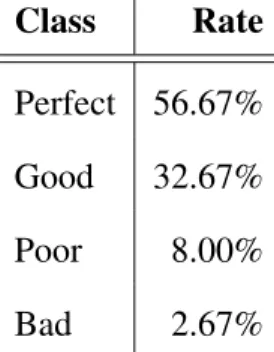
The outputs were classified into four classes according to the quality (%) of the result. The evaluation was done manually because an objective measure is hard to create.
• Perfect: the whole skyline [95−100%] is detected, no interfering fragments found.
• Good: the better part of the skyline [50−95%) is detected, false pixels do not affect the analyses.
• Poor: only a small part of the skyline [5−50%) is detected, false pixels might affect the analyses.
• Bad: skyline cannot be found or the detected edges do not belong to the skyline [0−5%).
Table 1 shows that the extracted skylines are assigned to Perfect or Good classes in more than 89% of the samples. In these cases, the extracted features can be used for matching in the next phase.
Class Rate
Perfect 56.67%
Good 32.67%
Poor 8.00%
Bad 2.67%
Table 1:Results of automatic skyline extraction method.
2.2.2 Results of Field Tests
We also made field tests to measure the performance of our algorithm in a real-world en- vironment. The experiments aimed to determine the orientation using only a geotagged photo and the DEM.
Table 2 presents the experimental results of the field tests. Only Good and Perfect skylines were accepted for the tests, and the correlation is almost 95% on average. These tests showed that the azimuth angles provided by the algorithm were 1.04◦ on an average from the ground truth azimuth.
6
Image Viewpoint Target Results
ID Lat (◦N) Lon (◦E) Height (m) Lat (◦N) Lon (◦E) Height (m) Corr. ϕ(◦) ϕˆ(◦) ϕˆ−ϕ(◦) FT01 47.51552 18.96866 330 47.55016 19.00178 436 0.92 31.58 32.60 1.02 FT02 47.51552 18.96866 330 47.53371 18.95588 429 0.96 334.62 334.61 -0.01 FT03 47.55555 18.99883 483 47.51827 18.95922 508 0.95 214.83 215.61 0.78 FT04 47.53154 18.98611 219 47.49178 18.97895 458 0.99 185.89 186.95 1.06 FT05 47.99865 18.86120 188 47.99564 18.86353 195 0.92 151.35 152.47 1.12 FT06 47.99948 18.86173 201 47.99564 18.86353 195 0.98 161.22 162.92 1.70 FT07 47.51827 18.95922 508 47.55016 19.00178 436 0.97 44.12 41.85 -2.27 FT08 47.98355 18.80440 124 47.95780 18.87714 723 0.88 118.98 118.58 -0.40 FT09 47.99865 18.86120 188 47.99564 18.86353 195 0.94 151.52 152.47 0.95 FT10 47.99948 18.86173 201 47.99564 18.86353 195 0.98 161.81 162.92 1.11
Table 2:Experimental results of the field tests.
3 Optimal Partisan Districting
In electoral systems with single-member districts or even with at least two multi-member districts, redistricting has to be carried out to resolve geographic malapportionment caused by migration and different district population growth rates. An inherent difficulty asso- ciated with redistricting is that it may favor a party. The problem becomes even worse if redistricting is manipulated for an electoral advantage, which is referred to as gerrymander- ing. A formal proof establishing that a simplified versions of the optimal gerrymandering problem is NP-complete were given by Puppe and Tasnádi (2009) and Lewenberg et. al (2017). Publication related to Section 3 is Fleiner et al. (2017).
3.1 The Framework
We assume that partiesA and Bcompete in an electoral system consisting only of single member districts. In addition, voters with known party preferences are located in the plane
and have to be divided into a given number of almost equally sized districts.
Definition 3.1. Adistricting problemis given byΠ = (X,N,(xi)i∈N,v,K,D), where
• X is a bounded and strictly connected2subset ofR2,
• the finite set of voters is denoted by N ={1, . . . ,n},
• the distinct locations of voters are given by x1, . . . ,xn ∈int(X),
• the voters’ party preferences are given v: N → {A,B},
• the set of district labels is denoted by K ={1, . . . ,k}, wherebn/kc ≥3, and
• D denotes the finite set of admissible districts consisting of bounded and strictly
connected subsets of X and each of them containing the location of bn/kcor dn/ke voters,and furthermore,
• we shall assume that based on their locations the n voters can be partitioned into k districts{D1, . . . ,Dk} ⊆ D.
Definition 3.2. An f : N → Dis adistrictingfor problemΠif there exists a set of districts D1, . . . ,Dk ∈ Dsuch that
• f(N)= {D1, . . . ,Dk},
• int(Di)∩int(Dj)=∅if i6= j and i, j∈K,
• {xi |i∈ f−1(Dj)} ⊂int(Dj)for any j ∈K.
3.2 Results
We establish that even the decision problem associated with the optimization problem of determining an optimal partisan districting, i.e., deciding for a given districting problemΠ whether there exists a districting with at leastmwinning districts for a party, say partyA, is an NP-complete problem. We call this WINNING DISTRICTS problem.
2We call a bounded subsetAofR2strictly connectedif its boundary∂Ais a closed Jordan curve.
8
Theorem 3.1. WINNING DISTRICTS is NP-complete.
The following easy consequence of Theorem 3.1 has practical importance.
Theorem 3.2. The decision problem whether a districting problem Πhas a districting in which party A gains majority is NP-complete.
3.2.1 A Positive Result
The problem becomes tractable if we replaceR2withRin Definition 3.1, i.e., if we restrict the two-dimensional problem to a one-dimensional one. Based on the dynamic program- ming technique, we develop a polynomial time algorithm that finds a so-called party A optimal districting for the one-dimensional districting problem.
3.2.2 A Practical Approach
We consider the Hungarian Electoral System in which since 2011, Budapest has to be subdivided into 18 electoral districts from a total of 1472 electoral wards, each serving 600- 1500 voters. Thus, an average district consists of approximately 82 wards. For simplicity, we model the election map by a 2-dimensional square grid, where every cell represents a ward with a given party preferenceAor B. In this model, two cells are connected if they share a common edge, so this defines a 4-neighborhood relation on the set of cells.
Even in this simplified structure, there is no known formula for the number of possible figures. It means, we do not know how many districts can be formed out of a given number of connected cells, so-called polyominoes. If even orientation matters, they are called fixed polyominoes. Jensen (2003) enumerated fixedn-cell polyominoes up to n = 56, which resulted in 6.9×1031 polyominoes for the last case. This result shows that it is unfeasible to examine all possible cases, even for 82 wards on a Budapest scale problem. Considering possible district shapes is just the first step in arriving to a districting.
Another starting point to obtain a heuristic for gerrymandering, i.e., an algorithm which is not optimal but quick, would be the pack and crack principle. We showed examples that the pack and crack principle does not always result in a partyAoptimal districting.
4 Circularity of Congressional Districts
Shape analysis has special importance in the detection of gerrymandering, the manipulated redistricting. Circularity is widely used as a measure of compactness, since it is a natural requirement for a district to be as circular as possible. We propose a novel circularity mea- sureM based on Hu moment invariants. This parameter-free circularity measure provides a powerful tool to detect districts with abnormal shapes. We also analyze the districts of Arkansas, Iowa, Kansas, and Utah over several consecutive periods and redistricting plans, and also compared the results with some classical circularity indexes (Reock (1961), Polsby and Popper (1991), and Lee and Sallee (1970)). Publications related to Section 4 are Nagy and Szakál (2019), Nagy and Szakál (2020).
4.1 Circularity Measures
Let us assume that all the examined shapes are compact in the topological sense. The following requirements hold for a circularity measureC:
1. C(D)∈(0,1] for any planar shapeD;
2. C(D)= 1 if and only ifDis a circle;
3. C(D) is invariant with respect to similarity transformations (translations, rotations and scaling);
4. For eachδ >0 there is a shapeDsuch that 0<C(D)< δ, i.e., there are shapes whose measured circularity are arbitrarily close to 0.
10
The following Proposition 4.1 and Definition 4.1 are from Žuni´c et. al (2010).
Proposition 4.1. Let D be a compact planar shape. Then
φ1(D)=η2,0(D)+η0,2(D)= µ2,0(D)+µ0,2(D) µ0,0(D)2 ≥ 1
2π
φ1(D)=η2,0(D)+η0,2(D)= µ2,0(D)+µ0,2(D) µ0,0(D)2 = 1
2π ⇐⇒ if D is a circle.
Based on Proposition 4.1 a circularity measureC1can be constructed as follows.
Definition 4.1. Let D be a compact planar shape and the area of circle O equals to the area of D. Then C1(D)is a circularity measure
C1(D)= φ1(O) φ1(D) = 1
2π · µ0,0(D)2 µ2,0(D)+µ0,2(D).
The following circularity measureCβ is a generalization ofC1, and it is applicable in special cases when we want to set the sensitivity manually for a specific purpose.
Definition 4.2. Let D be a planar shape whose centroid coincides with the origin and letβ be a real number greater than−1andβ6=0. Then Cβ(D)is the generalized moment-based circularity measure
Cβ(D)=
µ0,0(D)β+1 πβ(β+1)
Z Z
D
x2+y2β
dxdy
ifβ >0
πβ(β+1) Z Z
D
x2+y2β
dxdy
µ0,0(D)β+1 ifβ∈(−1,0).
We revealed an undesired feature of this measure, which emerged from the examined data. The circularity order can change when we apply differentβparameters to dissimilar shapes. Therefore, in the next definition, we propose the normalized measure of the area
under the curve ofCβ forβ ∈(−1,0)∪(0,∞) as a novel circularity measure and denote it byM.
Definition 4.3. Let Cβ(D)be the generalized moment-based circularity measure. Then M is a circularity measure
M(D)= lim
b→∞
1 b+1
Z b
−1
Cβ(D)dβ.
4.2 Results
We consider the average circularity of a state through successive Congresses and seek sig- nificant anomalies for gerrymandering detection. Thus, we can track the changes and re- duce the impact of external conditions, e.g., geographical constraints. We have analyzed four states in the period of the 107th, 108thand 113thUS Congress.
All circularity indexes of Utah decreased in stages from the 107thto the 113thCongress.
In Iowa, the examined indexes behaved similarly in these periods, the 107th showed the best, while 108th worst results. In Arkansas, Lee-Sallee Index and Polsby-Popper Test decreased monotonically while Reock Test and M had a peak at 108th. Remarkably, M was more sensitive to the change than Reock Test. The most interesting state was Kansas, where the indexes gave completely different orders, and Mwas the only one with a falling trend.
An example of presumable gerrymandering is the third district of Arkansas through the 107th, 108thand the 113th Congress. We can see an almost unambiguous improvement in the circularity values from the 107th to the 108th period, then a significant fall from the 108thto the 113thCongress.
12
5 Publications of the Author
Fleiner, B., Nagy, B., and Tasnadi´ , A. (2017), Optimal partisan districting on planar geographies,Central European Journal of Operations Research25, 879–888.
Nagy, B. and Szak´al, Sz. (2019), Választókerületek alakjának vizsgálata Hu-féle invariáns momentumok alkalmazásával, Alkalmazott Matematikai Lapok 36, 161–
183.
Nagy, B. (2020), A new method of improving the azimuth in mountainous terrain by skyline matching,PFG - Journal of Photogrammetry, Remote Sensing and Geoinfor- mation Science88, 121–131.
Nagy, B. and Szak´al, Sz. (2020), Measuring the circularity of congressional districts, Society and Economy42, 298–312.
References
Blum, J., Greencorn, D., and Cooperstock, J. (2013), Smartphone sensor reliability for augmented reality applications,Proceedings of the 9th International Conference on Mo- bile and Ubiquitous Systems: Computing, Networking and Services, 127–138.
Fedorov, R., Frajberg, D., and Fraternali, P. (2016), A framework for outdoor mobile augmented reality and its application to mountain peak detection, Augmented Reality, Virtual Reality, and Computer Graphics, 281–301.
Jensen(2003), Counting polyominoes: A parallel implementation for cluster computing, International Conference on Computational Science, 203–212.
Lee, D. and Sallee, T. (1970), A method of measuring shape, American Geographical Society, Wiley60, 555–563.
Lewenberg, Y., Lev, O., and Rosenschein, J. (2017), Divide and conquer: Using geographic manipulation to win district-based elections,Proceedings of the 16th Conference on Au- tonomous Agents and MultiAgent Systems, 624–632.
Polsby, D. and Popper, R. (1991), The third criterion: Compactness as a procedural safe- guard against partisan gerrymandering,Yale Law&Policy Review9, 301–353.
Puppe, C. and Tasnadi´ , A. (2009), Optimal redistricting under geographical constraints:
Why “pack and crack” does not work,Economics Letters105, 93–96.
Reock, E. (1961), A note: Measuring compactness as a requirement of legislative appor- tionment,Midwest Journal of Political Science5, 70–74.
Zhu et. al. (2012), Skyline matching: A robust registration method between Video and GIS,Usage, Usability, and Utility of 3D City Models–European COST Action TU0801, 03007
Žuni´c, J., Hirota, K., and Rosin, P. (2010), A Hu moment invariant as a shape circularity measure,Pattern Recognition43, 47–57.
14