Economic preferences in the classroom - research documentation
Dániel Horn(a)(b), Hubert János Kiss(a)(b), Tünde Lénárd (a) May 30, 2020
Abstract
In this paper, we document how we carried out a research that aimed at measuring the economic preferences of high school students. We describe the preferences that we study and what experimental games we used to investigate them. Then we report how we carried out the experiments in the schools. We provide detailed descriptive statistics on the preferences in aggregate and also school by school. Last, we validate our measurement by comparing the measured preferences to those in the literature.
Keywords: altruism, competitive preferences, cooperation, risk preferences, social preferences,
student, time preferences, trust
JEL codes: C70, C80, C90, D91, J16
Funding: The project received funding from the Hungarian National Research, Development and Innovation Office, grant number K-124396.
(a) Institute of Economics, Centre for Economic and Regional Studies, Budapest, Tóth Kálmán utca 4, H-1097, Hungary
(b) Corvinus University of Budapest, Hungary
1 Introduction
From March 2018 to March 2020, we visited 10 secondary schools in Hungary to measure the economic preferences of students. This paper documents how we carried out the measurements, what issues arose and how we solved them. We also present detailed descriptive statistics and perform a validation exercise. Overall, we measured time, risk, social and competitive preferences of 1276 students in 71 school classes (groups of students studying the major subjects together). As we will show, the correlations between the measured preferences and the associations between the preferences and socio-demographics of the students are in line with those reported in the literature.
The project has been funded by the National Research and Development Office of Hungary (project no. 124396). The experiments were run in Hungarian, and also the related legal documents are available in Hungarian here: https://www.mtakti.hu/kapcsolat/altalanos-tajekoztato-a- kiserletekrol/.
The experiments were anonymous, but we can link the individual preferences with the individual data from the National Assessment of Basic Competences (NABC) – see more details below – which allows us to see how preferences relate to individual school performance, aspiration and other school characteristics (type of class, curriculum, location, etc.). It also provides us with useful information about the participants’ family background. With the detailed preference map of the students and the additional information on their family background and school performance, we want to study several research questions. For instance, we are interested in the distribution of preferences between and within schools, how family background associates with preferences, the association of past school performance and recent preferences, the mediating power of family between past school performance and preferences. Since we have school-class level data, we can also study if classes with better aggregated social preferences perform better academically. That is, do classes where students are more generous, cooperative and trusting exhibit better academic results?
In this report, we present only the descriptive statistics of the data that we have collected and defer the more detailed statistical and econometric analysis to future research papers.
2 Preferences and experimental games
In the last decade, the study of adolescents’ preferences has become a very intense field, mostly aiming to understand how those preferences affect school performance and behaviour or later life outcomes. Most of the studies in this literature focus only on a limited set of preferences (see Sutter et al. 2019, for a survey of the literature). If the preferences are correlated, then a separate measurement of them and inferences drawn from those measurements may lead to incorrect conclusions. For instance, the measurement of time preferences involves the choice between amounts of money to be received at different points in time. However, since the future is inherently risky, these intertemporal choices may be affected by risk preferences as well. Similarly, entering a competition is a risky choice. People, who are risk-averse, might be opting out from competitive situations, even if they would not shy away from competition, ceteris paribus.
Our goal was to obtain a more comprehensive picture of the preferences of the participants.
Therefore, we chose to measure the most basic and widely studied preferences: time, risk, social and competitive preferences. Social preferences include generosity (also known as altruism), cooperation and trust. Overall, students participated in 8 experimental tasks, so we have a detailed dataset that allows us to obtain a fairly accurate map of preferences. With this set of preferences, it is possible to pin down the effect of separate preferences because we can control for the effect of the other ones.
2.1 Procedures
We conducted our computer-based experiment in 71 classes in 10 schools. Before starting the project, we contacted all educational providers in Hungary with at least one secondary school (academic, vocational or mixed) to request permission to run the experiment in their institutions.
Providers with only Special Vocational Schools were left out (see Lénárd, Horn and Kiss 2020).
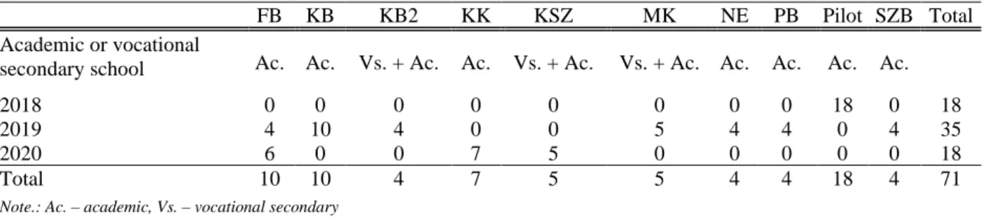
The schools included in our sample were either suggested by the provider or – given the positive feedback from their provider – they voluntarily indicated their willingness to participate. Five of them operate in Budapest and five in smaller rural towns of Hungary. To maintain the anonymity of the schools, we use acronyms, see Table 1.
FB KB KB2 KK KSZ MK NE PB Pilot SZB Total
Academic or vocational
secondary school Ac. Ac. Vs. + Ac. Ac. Vs. + Ac. Vs. + Ac. Ac. Ac. Ac. Ac.
2018 0 0 0 0 0 0 0 0 18 0 18
2019 4 10 4 0 0 5 4 4 0 4 35
2020 6 0 0 7 5 0 0 0 0 0 18
Total 10 10 4 7 5 5 4 4 18 4 71
Note.: Ac. – academic, Vs. – vocational secondary
Table 1. School classes by school and year
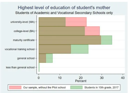
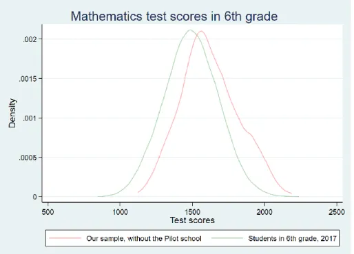
Naturally, our sample of schools is not representative of the total school population of Hungary, as we went mainly to academic tracks and a few vocational secondary schools (offering maturity exams). Figures 1 and 2 compare our sample to the whole universe of such schools in Hungary in terms of socioeconomic status (captured by the highest level of education of the mother) and gender composition. Figure 3 compares 6th-grade math test scores of the students in our sample to the test scores of 6th grade students in 2017.
Figure 1 shows that the socioeconomic status of the students that participated in our experiments is higher than that of the whole population as the share of students in our sample who have a mother with a tertiary degree is higher than the same share in the population.
Figure 1. Distribution of highest level of education of student’s mother in our sample and the population
Figure 2 shows that in terms of gender composition, the share of females is somewhat higher in our sample than in the population, but the difference is not pronounced.
Figure 2. Distribution of gender in our sample and the population
Figure 3 reveals that the mathematics test scores measured by the National Assessment of Basic Competences in 6th grade are on average higher in our sample than they are in the population of all 6th-grade students in 2017.1
Figure 3. Distribution of test scores in 6th grade in our sample and the population
The experiments were conducted during school hours, with each session being roughly as long as a regular lesson. Since we went to the schools and carried out the experiment there, we had to adapt to the time schedule of the schools. In most Hungarian schools, classes are 45 minutes long, followed by a 15-minute long break. Thus, we had 45 minutes (at most 60 minutes) to run the experiment with a class.
Participation was voluntary and anonymous. We sent out the data protection statement to all parents and children prior to the assessment, notifying them that in our survey we ask for the students’ IDs used at the National Assessment of Basic Competences (NABC) which allows us to connect our experimental data to anonymous NABC data on school performance and socioeconomic background at the individual level. Only two students have opted out from our experiments. The NABC ID is a hash-code of the educational IDs of the students, and is used only
1 The difference is significant (t-test, p<0.0001).
to identify students within the NABC surveys but are otherwise not linked to any other datasets.
Education providers had also been notified that we would collect NABC IDs, and none of them protested against this practice.
We asked the schools to distribute the NABC IDs to the students before the experiment on paper, which they had to take away after. Students could only start the experimental games after typing in their IDs, but no other individual data were asked.2
Participants were classmates in all sessions, which is an important feature in our experiment that allowed us to measure in-group and out-group favouritism (see section 2.4.1) as well as other class-level characteristics. Some of the tasks were individual tasks, where payoffs did not depend on the choices of other participants. Other tasks involved strategic interaction, so the decisions of two participants determined the payoffs. In these cases, the software that we used to program the experiment (z-Tree, Fischbacher (2007)) created student pairs randomly. Pairing always occurred at the end of the experiment, after obtaining information about each student’s decision in each hypothetical situation. When we had an odd number of participants in the room, then the last „pair”
of students was a group of three participants. In games that required interaction, the payments of students in the group of three were affected by the decision of only one of the other students in that group. This was also randomly determined by the program.
We used meal vouchers for the school cafeterias to incentivize the experiments. We explained to students that they would make decisions in 8 tasks, and at the end of the experiment, one of the tasks would be chosen randomly by the computer for payment (same for everyone in a session). Many of the tasks involved more choices. We made clear that in these cases, one of those choices would be picked randomly for payment. All sums were rounded to hundred Forints (the Hungarian currency) as we paid out the students in hundred Forints. There was no show-up fee, as
2 There were some problems of the distribution of the NABC IDs in some classes in our sample. These groups got temporary IDs, so we are not able to link their preference data to the NABC database, hence some background data is missing.
we have visited students in their school. We designed the payoffs so that the expected payoff would be around 1000 HUF (around 3 EUR).3
Participants were informed about the payout details (e.g. random selection of tasks and decisions for payment) right before each session and were paid after everyone in their school group had finished all tasks. If one of the two time-preference tasks was selected for payment (in which students had to choose between different sums of money paid at different times), everyone was paid according to their individual decision. The sums requested at the time of the experiment were handed out after the experiment. Students who chose to have another amount two, four or six weeks later had to put their vouchers in an envelope, which we placed at the school secretariat asking the management of the school to give out these vouchers two, four or six weeks later (as indicated on each envelope).4
On experiment day, we unpacked our laptops in the school in a designated classroom, turning it into our laboratory for the day. Participants used school computers in only two Budapest schools, which also meant using a mouse instead of a touchpad. In all the other cases, it was easier to bring our laptops with the necessary programs and settings, as schools have typically no or smaller labs.
When participants entered the room where we carried out the experiment, they were free to choose a seat. They had a sheet with the instructions in front of them. Once everybody seated, an experimenter read aloud this instruction sheet. Any questions from the students were answered.
A shorter version of the rules appeared on the start screen of the experiment. Participants were assured that all decisions remained confidential.
3 1000 HUF is around the cost of a full meal at a school cafeteria.
4 We were careful to choose dates for the experiments so that payments in 2,4 or 6 weeks can be received and that the vouchers could be used without any problem. That is, no later payment occurred during holidays. Note however, that the Covid-19 outbreak has impacted some of the later payments. We have agreed with the schools to distribute these later payments for the students when normal routine returns. Note also, as the outbreak and the imminent school closure was unexpected, this should not have affected the choices the students made.
We did not impose time limits in the different tasks (except the real-effort task to measure competitiveness, see below) so the participants could take their time. The only constraint, as mentioned, was that we had to end the experiment before the next class. We also explained to the participants that potentially there could be large differences in how much it would take for different participants to choose in different tasks, and we asked them to be patient. In fact, there was large heterogeneity in the time that participants spent with the games, but we had no incidents due to having to wait for the others who needed more time to decide.
In all occasions, at least two experimenters were in the room to monitor if everything went smoothly. In the instructions, we warned the participants that we did not tolerate misbehaviour (speaking to others, looking at their screens etc.) and that such behaviour could be punished with expelling the misbehaving participant without any payments. Fortunately, no such punishments were needed, there was no major incident related to misbehaviour during the experiments.
It has not been obvious in which order our 8 tasks should be performed. We took into account the following considerations when establishing the order. We wanted to have the two time preference tasks apart, as participants might have unwittingly tried to be consistent by making the same choices had the two tasks been neighbouring. Since the two dictator games involved the same decision but with different reference groups, we put these questions close to each other. The only task that could have affected the emotions of the participants more intensely was the competitiveness task, as participants were placed in a competitive setup that some of them may not have liked. Moreover, feedback on their performance after each round were provided. In order to avoid that the experience in this task affects the choices in other tasks, we put the competitiveness task at the end. Regarding the rest of the experimental tasks, we did not give feedback to the participants between tasks to avoid that the outcome of a task affects choice in the subsequent tasks.
To test if we can carry out the experiment properly, in March 2018, we went to the Pilot high school where we tested 18 different classes/groups of students, with differing sizes. Using this experience, we altered two of the initial experimental tasks. The first concerned the measurement of risk preferences that in the pilot were measured following Falk et al. (2018) gamble games, using the staircase method. Since gambles were not so natural for our subject pool, for the subsequent schools we opted for using the bomb risk elicitation task (Crosetto and Filippin 2013) that involves a story about a risky choice and seemed more appropriate for high school students. The other change was in the competitiveness task, where we changed the real-effort task.
In the pilot, we used the slider task (Gill and Prowse 2019), but it was susceptible to the computer that participants used and participants with more computer experience performed better (mainly due to playing computer games). Hence, the task was not neutral enough for our purpose. Instead of this task in the rest of the schools, we used a different real-effort task consisting of counting zeros and ones in 5x5 matrices (see Abeler et al. 2011).
After each visit, we sent feedback to the schools.5 We explained briefly in the feedbacks, what preferences the different tasks measured, and we reported the main descriptive statistics, comparing them to the main findings of the literature. We also compared succinctly how different school groups performed.
2.2 Time preferences (task 1 and 6)
Time preferences express how an individual trades off earlier and later benefits and they are generally measured with choices that individuals make between an earlier and a later amount of money (see Andreoni et al. 2015; Cohen et al. 2016).
Time preferences have at least two relevant aspects. Patience reveals how an individual values the future relative to the present, while time consistency indicates if this relative valuation
5 In case of two high schools in Budapest, they invited us to give a short presentation to the participants and the teachers.
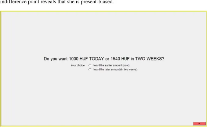
is the same at different points in time. Patient individuals value the future more relative to the present than their less patient peers. Time consistent individuals trade off earlier and later benefits in the same way at different points in time. In contrast, present-biased (future-biased) individuals are less (more) patient in the near future than later on. To capture both aspects of time preferences, we needed two different time horizons. Our participants had to choose between receiving a smaller amount today or a larger amount in 2 weeks (task 1) and they faced the same situation, but the dates were 4 weeks vs. 6 weeks (task 6). On both horizons, participants had to make 5 interdependent choices, following the staircase (or unfolding brackets) methodology (Cornsweet 1962). This methodology uses the available number of questions efficiently to zoom in on the indifference point between the earlier and the later payoffs. In each case, the earlier amount was fixed (1000 Ft) while the later amount (X) was changed adaptively, depending on the previous choices. For example, if a participant chooses 1000 Ft today instead of X=1540 Ft in 2 weeks, then we know that her indifference point is higher than 1540 Ft, so in the next question X is increased.
Similarly, the choice of the later amount implies a decrease in X in the next question. X varied from 1030 to 2150 Ft. Five questions allow a reasonable approximation to the indifference point, so we know how much we have to offer so that the participant is willing to wait 2 weeks to receive the payment.6 Suppose that a participant in task 1 (today vs. 2 weeks) in the last question chooses to receive 1730 Ft in 2 weeks instead of 1000 Ft today. Then (by the construction of the payoffs) we know that her indifference point is between 1730 Ft and the closest lower amount (1650 Ft).
For practical reasons, in this case, we consider that her indifference point is 1650, so she needs a 650 Ft compensation for waiting 2 weeks to receive the payment.7 If the same participant in task
6 In Appendix B we represent graphically the map of the five choices that participants may have faced during this task.
7 We chose to proxy time preferences by the lower bound because if a participant is very impatient and always chooses the immediate 1000 Ft, then we know that her indifference point is above 2150 Ft, but we do not know how much above it. Therefore, considering the lower bound allows us to be consistent, but admittedly we underestimate somewhat the indifference point. Choosing the midpoint between bounds or the upper bound would not change our findings qualitatively.
6 (4 weeks vs. 6 weeks) has the same indifference point, then she is time consistent, while a lower indifference point reveals that she is present-biased.
Figure 4. Screenshot from the first time preference task (now vs. 2 weeks)
There was also a 6th choice in both time preference tasks to check the rationality and / or thoughtfulness of the participant. In this choice, the later amount either was very high (3000 Ft, which is triple the amount of the immediate payment) or lower than the earlier amount (900 Ft). If a participant chooses always the earlier 1000 Ft instead of the later, but larger amounts, including 3000 Ft 2 weeks later, then it implies an extraordinarily high discounting of the future, which we considered an outlier. Choosing a later 900 Ft instead of an earlier 1000 Ft indicates negative discounting which seems to be extreme. Hence, with these control questions, we can identify participants who have very extreme time preferences or do not take the experiment seriously.
We explained to participants that if this task is chosen for payment, then one of the first 5 decisions would be picked randomly by the computer and their choice in that decision would be implemented. For example, if a student chooses 1540 Ft in two weeks instead of 1000 Ft today, then she would receive the 1540 Ft in two weeks from the school administration as we explained above.
The time preference tasks measure the amount of money to be received two weeks later that makes a participant indifferent to receive 1000 Ft earlier. We will call these amounts Indifference amount now (based on choices between amounts now or in 2 weeks) and Indifference amount 4 weeks (based on choices between amounts in 4 weeks or in 6 weeks), and we will report the averages later in the paper. Larger indifference amounts indicate less patience.
2.3 Risk preferences (task 4)
Risk preferences indicate how an individual approaches a choice that has an uncertain outcome. Therefore, the tests to measure risk preferences involve some situation with uncertainty.
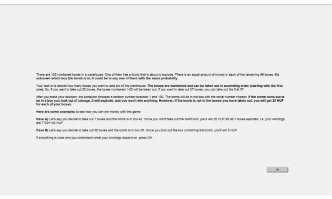
Many of these tests include gambles (e.g. Eckel and Grossman 2002, Gneezy and Potters 1997, Holt and Laury 2002) that may seem strange to our student pool as evidenced by our experience in the Pilot high school, so we decided to use the bomb risk elicitation task by Crosetto and Filippin (2013). In this task, the participants are presented with the following short story. There is a store with 100 numbered boxes, one of which contains a bomb. The bomb can be in any of the boxes with the same probability. Participants have to decide how many boxes they want to collect, but the boxes can only be obtained in the order of their numbering. Earnings increase with the number of boxes collected that do not contain the bomb, but participants earn zero if the bomb is in one of their boxes. The number of boxes participants are willing to collect is a proxy for risk preferences.8
8 Crosetto and Filippin (2016) compare four risk elicitation methods that are widely used in experimental economics, among them the bomb risk elicitation method and find that it is a valid measure of risk preferences.
Figure 5. Screenshot of the risk preference task
Participants knew that if this task was selected for payment, the computer would choose a random number between 0 and 100 indicating the box that contains the bomb. If the number of boxes that the participant decided to collect was below that number, then she would earn 20 Ft for each box. Otherwise, her earning would be zero. We will report the average of boxes that participants decided to collect (Risk-taking: # of boxes), larger numbers indicating more risk tolerance.
Choosing 100 boxes is equivalent to a sure explosion and zero earnings. We set the risk- taking measure to missing if the student took 100 boxes.
2.4 Social preferences
Social preferences have many aspects. In our experiment, we focused on three: generosity, cooperativeness and trust.
2.4.1 Generosity (task 2 and 3)
We measured generosity (or altruism) with the dictator game. There were two dictator games. In the first one (task 2) we endowed all participants with 2000 Ft that they could split
between themselves and somebody else in the room, that is one of the classmates. We explained to participants that if at the end of the experiment this task was payoff-relevant, then we would pair the participants randomly. In each pair, the computer would randomly select one of the participants whose decision would be implemented. In task 3, we repeated this game, but this time the co-player was not somebody from the room, but a random schoolmate. This task was hypothetical.
Figure 6. Screenshot of the dictator game
We will report the sum given to the classmate (Giving to classmate) and to the schoolmate (Giving to schoolmate), larger sums denoting more generosity.
2.4.2 Cooperativeness (task 5)
The second aspect of social preferences that we measured was how cooperative our participants were. We used the workhorse test of cooperation, the public goods game (task 5).
However, instead of forming groups of 4 as is usual in most experiments with the public goods game, we applied a two-person variant. That is, we paired each participant randomly with somebody else from the room. Both of them were endowed with 1000 Ft, and they had to decide how much of the endowment to contribute to a common account, without knowing the contribution
of the other participant. The amount that they did not contribute to the common project was theirs.
From the common project, each of the two participants received 75% of the total contributions, independently of the individual contribution. Our measure of cooperativeness is the contribution to the common project: the more a participant contributes, the more cooperative she is.
To make the decision easier, on the decision screen, below the description of the task, participants had two sliders, both of them going from 0 to 1000, the first corresponding to their contribution and the second corresponding to their co-player’s contribution. By using the sliders, they could see the payoff consequences of different contribution combinations (see the decision screen in Figure 7).
Figure 7: Screenshot from the cooperativeness task (public good game)
We will report the contribution to the common project (Cooperation: contribution), larger values implying higher levels of cooperativeness.
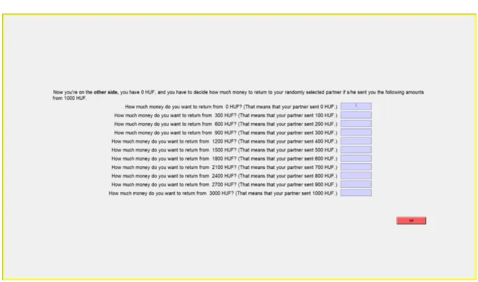
2.4.3 Trust (task 7)
We used the trust game (also known as investment game by Berg et al. 1995) to measure trust and trustworthiness of the participants. The game had two steps. In step 1, each participant played the role of the sender. They started with an endowment of 1000 Ft, and they decided how
much to send to a randomly selected co-player in the room. The sum that they chose to send is a measure of trust. We told explicitly that the sum would be rounded to the nearest 100. In step 2, the sent amount tripled. Here everybody assumed the role of the receiver and they had to state how much they would send back of the 3*X if the sender had sent them X (X={0,100,200,...1000}) Ft.
Thus, we have answers to all contingencies, and this profile of responses provides a proxy of trustworthiness.
Figure 8. Screenshot from the second part of the trust game
We explained to the participants that if this task were chosen for payment, then the computer would form random pairs in the room and one player in each pair would be randomly chosen as sender and the other as a receiver and their corresponding choices would determine the payment.
We will report the sum that the participants sent (Trust: sum sent) and also the average percentage of the received sum that the participant returned (Trust: % returned). Higher values indicate more trusting/trustworthy participants.
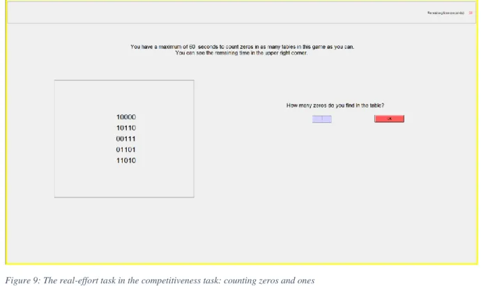
2.5 Competitiveness (task 8)
In the last task of the experiment, we used the Niederle and Vesterlund (2007) setup to measure competitiveness.9 The only change that we made was to use a different real-effort task.
Instead of adding up numbers, participants had to count zeros and ones in 5x5 matrices (for instance, in Abeler et al. 2011). Figure 4 shows a screenshot of the counting exercise. In each stage of the game, they had 1 minute to carry out the task.
The game started with the piece-rate stage in which participants were paid based on the number of correctly solved matrices, each paying 100 Ft. In stage 2, participants were evaluated as if they participated in a tournament, only the best 25% of the participants in the room earning money for the task.10 However, their earnings were 4 times as high per matrix solved as in stage 1. In stage 3, participants could choose if they wanted to get paid according to piece-rate or tournament, their choice indicating if they were competitive or not. After stage 3, we asked participants how they ranked themselves (being in the 1st / 2nd / 3rd / 4th quartile) based on their performance in stage 1 (piece rate) and stage 2 (tournament). These beliefs were elicited in an incentivized way as those who guessed correctly received 300 Ft (if this task was chosen for payment).
At the end of the experiment, if the computer chose this task for payment, the computer picked one of the stages randomly and participants were paid according to their performance in that stage.
In our descriptive tables, we will report the share of competitive participants (Competitive).
9 Lise Vesterlund was very kind to share with us their z-tree code for which we are grateful.
10 In case of tie, the computer randomly decided who got into the 25% to be paid.
Figure 9: The real-effort task in the competitiveness task: counting zeros and ones
3 Descriptive statistics
The full sample consists of 1276 students from 8th to 12th grades (8th grade: 41 students; 9th grade: 418 students; 10th grade: 385 students; 11th grade: 336 students; 12th grade: 96 students). 56
% of all participants were female.
We gained all student-level information – asides the economic preferences – from the National Assessment of Basic Competencies individual database. Gender and age data are missing only for a very few cases, but for 11% of the cases, socioeconomic status values are missing as these were self-reported in the NABC questionnaire.
As risk and competition preferences were measured differently in the Pilot school, descriptive statistics are shown without the pilot data.11 Table 2 shows the descriptive statistics of all raw preference measures that we have collected. We did not use the time preference measures of those students who gave an extreme or thoughtless answer to our control question (see section
11 We report the descriptive statistics of the preferences measured in the Pilot school in section 3.1.
2.2). We also did not use the risk-taking measures of those who chose to take 100 boxes out of the 100.
Students earned around 1000 HUF on average with a standard deviation of around 800 HUF (note that depending on the type of the game that was chosen for payment and the decisions of the students, the final profit varied between 0 and 6400 HUF).
Variable N Mean SD Min Max
Female 1036 0.56 0.50 0.00 1.00
Age 1035 16.93 1.14 14.00 21.00
School grade 1108 10.11 0.95 9.00 12.00
Final profit 1108 1038.99 831.70 0.00 6400.00
Indifference amount now 1077 1410.58 406.86 1030.00 3000.00 Indifference amount 4 weeks 1089 1414.15 344.87 1030.00 3000.00
Risk: # of boxes 1100 33.62 18.52 1.00 99.00
Risk, female 578 30.94 18.25 1.00 99.00
Risk, male 450 37.38 18.64 1.00 99.00
Giving to classmate 1108 783.66 370.18 0.00 2000.00
Giving to schoolmate 1108 554.69 412.22 0.00 2000.00 Cooperation: contribution 1108 605.13 275.12 0.00 1000.00
Trust: sum sent 1108 551.81 253.69 0.00 1000.00
Trust: % returned 1108 38.82 16.45 0.00 100.00
Competitive 1108 0.61 0.49 0.00 1.00
Competitive, female 583 0.56 0.50 0.00 1.00
Competitive, male 453 0.66 0.47 0.00 1.00
Table 2. Descriptive statistics without the pilot data
Table 2 also reveals that students required approximately 400 extra Ft for having to wait two weeks to receive their payments, both when the choice was now vs 2 weeks and 4 vs 6 weeks.
In the task measuring risk preferences, students collected on average 34 boxes which is somewhat lower than the literature reports (see Crosetto and Filippin 2013). Male participants collected more boxes than females which is an indication of higher risk tolerance, an often found gender difference in preferences (e.g. Croson and Gneezy 2009, or Bertrand 2011). Students were more generous toward their classmates than toward their schoolmates (who received about 28% of the endowment), giving more than 200 Ft (10% of their endowment) more to them. Participants contributed on average 60% of their endowment to the common project in the task measuring cooperation, which corresponds to the higher end of the findings in the literature (see Chaudhuri 2011). Similarly, the 55% that participants sent in the trust game is somewhat higher than the 50%
observed in the literature (see Johnson and Mislin 2011). Being more cooperative and trusting is
not surprising as in our experiment participant played with their classmates and not with strangers.
In line with the literature, we also find that males are more competitive than females (e.g. Niederle and Vesterlund 2011). Overall, the main descriptive statistics are in line with those found in the literature.
Table 3 shows the average preference measures by school. In some tasks, most of the schools exhibit similar average behaviour (e.g. sum returned in the trust game), but there are also big differences in other dimensions. For instance, in school MK students on average are much more impatient than their peers in school PB as they require more than 20% more money for having to wait two weeks (see row Indifference amount now).12
School code Pilot FB KB KB2 KK KSZ MK NE PB SZB Means
without Pilot
Subject 167 253 149 65 166 105 98 103 99 70
Female 0.53 0.39 0.65 0.90 0.66 0.66 0.55 0.56 0.56 0.41 0.56
Age 16.42 16.38 17.83 15.98 16.48 19.30 16.74 17.44 16.45 17.32 16.93
Indifference amount now 1352.50 1340.29 1451.22 1506.45 1380.43 1366.83 1569.57 1485.05 1297.08 1459.41 1410.58 Indifference amount 4 weeks 1315.94 1307.76 1400.75 1538.44 1479.26 1443.24 1505.81 1447.50 1353.67 1428.84 1414.15 Risk-taking 47.38 41.07 33.68 26.40 29.70 31.74 30.14 35.69 32.20 29.38 33.62 Risk, female 51.20 39.07 32.05 26.91 27.06 29.73 28.35 34.57 28.49 27.07 30.94 Risk, male 43.16 42.35 36.39 27.50 34.91 38.00 32.34 36.76 37.21 31.10 37.38 Giving to classmate 892.76 705.51 862.68 851.54 808.76 869.10 852.76 654.61 735.36 808.64 783.66 Giving to schoolmate 649.72 493.11 629.60 610.77 575.87 630.24 630.78 458.20 489.05 530.43 554.69 Cooperation: contribution 630.95 660.98 626.85 510.29 573.86 628.30 603.63 587.73 595.18 526.29 605.13 Trust: sum sent 634.73 618.18 573.15 478.46 504.82 544.76 528.57 549.51 546.46 500.00 551.81 Trust: % returned 42.00 36.61 42.01 35.52 37.84 40.12 42.34 37.25 37.60 42.50 38.82
Competitive 0.67 0.55 0.64 0.52 0.61 0.69 0.61 0.59 0.61 0.76 0.61
Competitive, female 0.65 0.50 0.59 0.53 0.53 0.64 0.57 0.60 0.52 0.79 0.56
Competitive, male 0.70 0.56 0.75 0.33 0.79 0.88 0.66 0.58 0.69 0.73 0.66
Note: Risk-taking means gamble games with staircase method in the Pilot school, bomb risk elicitation task in all other schools
Table 3. Raw averages by school
The aggregate school-level data suggest that there is considerable heterogeneity between schools in the preferences that we measured. 13 Table 4 shows the z-standardized scores of all preferences measures (with 0 mean and 1 standard deviation). As we will show later, there is also considerable heterogeneity in preferences within schools.
12 Note also that on the other hand students on average are more generous in school MK than in school PB.
13 The high values in the risk-taking task in the Pilot school may be due to the fact that there we used a different task.
We converted the measure used there so that the numbers are comparable and we represent them for sake of completeness.
School code Pilot FB KB KB2 KK KSZ MK NE PB SZB
Indifference amount now -0.13 -0.16 0.12 0.26 -0.06 -0.09 0.42 0.21 -0.27 0.14
Indifference amount 4 weeks -0.25 -0.28 0.00 0.41 0.23 0.12 0.31 0.14 -0.14 0.08
Risk-taking 0.63 0.30 -0.09 -0.47 -0.30 -0.19 -0.28 0.01 -0.17 -0.32
Risk, female 0.92 0.29 -0.08 -0.34 -0.33 -0.20 -0.27 0.05 -0.26 -0.33
Risk, male 0.27 0.22 -0.10 -0.57 -0.18 -0.01 -0.31 -0.08 -0.05 -0.38
Giving to classmate 0.26 -0.25 0.18 0.15 0.03 0.19 0.15 -0.39 -0.17 0.03
Giving to schoolmate 0.20 -0.18 0.15 0.11 0.02 0.15 0.15 -0.26 -0.19 -0.09
Cooperation: contribution 0.08 0.19 0.07 -0.35 -0.12 0.07 -0.02 -0.07 -0.05 -0.30
Trust: sum sent 0.28 0.22 0.04 -0.33 -0.23 -0.07 -0.13 -0.05 -0.06 -0.25
Trust: % returned 0.17 -0.16 0.17 -0.23 -0.09 0.05 0.19 -0.12 -0.10 0.20
Note: Risk-taking means gamble games with staircase method in the Pilot school, bomb risk elicitation task in all other schools
Table 4. Z-standardized averages by school
Table 4 reports averages, but the whole distribution of preferences may provide interesting insights into the heterogeneity of preferences between schools as well. In Figures 10-17 we show boxplot graphs that illustrate how dispersed the observations are school by school.14
Figure 10. Heterogeneity of the preference measures – Indifference amount now
Figure 10 indicates that extra money needed to make a student indifferent between receiving the money now or in two weeks is much more dispersed in some schools than on others.
For instance, in schools FB, KSZ and PB the indifference amounts are not only lower on average, but they are also more concentrated than in schools KB2, MK or NE. Figure 11 shows similar patterns for the other time preference task.
14 The horizontal line within the box represents the median, while the bottom / top of the box indicates the 25th / 75th percentile of the observations. The upper (lower) adjacent value is the 75th (25th) percentile plus (minus) 3/2 times the interquartile range.
Figure 11. Heterogeneity of the preference measures – Indifference amount 4 weeks
Note: Risk-taking means gamble games with staircase method in the Pilot school, bomb risk elicitation task in all other schools
Figure 12. Heterogeneity of the preference measures – Risk-taking
Figure 12 reveals that even though the average number of boxes collected in the bomb risk elicitation task (our risk measure) differ considerably across schools, the distributions do not seem very different.
Figure 13. Heterogeneity of the preference measures – Giving to classmate
Figure 14. Heterogeneity of the preference measures – Giving to schoolmate
Figure 13 indicates that regarding Giving to classmate not only the average amounts differ across schools, but also the dispersion of the data. In schools KSZ, MK and Pilot students are not only more generous on average to their classmates, but in these schools, most of the students are similarly generous to each other. Figure 14 demonstrates that when it comes to giving to a random schoolmate, generosity declines, and it also becomes more dispersed.
Figure 15. Heterogeneity of the preference measures – Cooperativeness
Figure 15 uncovers heterogeneity across schools in cooperativeness. In schools where the average contribution is low, the distribution tends to be less spread out than in schools with higher averages.
Figure 16. Heterogeneity of the preference measures – Trust: sum sent
Heterogeneity is also present in trusting behaviour as exemplified by Figure 16. Averages do not differ much across schools, but clearly, the decisions are more dispersed in some schools than others.
Figure 17. Heterogeneity of the preference measures – Trust: sum returned
Figure 17 shows that concerning the share of money returned to the sender, we do not see much heterogeneity across schools.
Although the previous figures suggest that there is some heterogeneity across schools, but it also shows that there is considerable overlap in behaviour across schools. In Appendix C we show probability density functions (both pooling all schools in one graph and separately) that expose the degree of similarity of behaviour across schools as it is hard to distinguish the probability density functions in many cases. These functions also illustrate the presence of focal points in many measures (e.g. giving or contribution 500 or 1000 Ft-s).
3.1 Pilot school
First, we ran the pilot version of the experiment. 168 students from 18 school groups participated in the study. All groups were academic classes, and 53% of the students were female.
This school operates in Budapest. A unique feature of this school is that the school groups are
rather small, comprising less than 20 students on average. Due to technical difficulties, zTree did not save the data properly at the end of session 2 (Group 2), and we were only able to recover the output partially. The final data loss did not affect the main variables presented in Table 5.
As reported in Table 5, most of the groups were more patient than the average of the full sample as they required less than 400 HUF for having to wait two weeks now or a month later.
Regarding risk-taking, students were well above average, and in most groups, male students were more risk-averse than female students which is the opposite of what we observe in other schools.
This might be due to the fact that in the Pilot school, we used a different (gambling) game for measuring risk aversion than in the other institutions. There is considerable heterogeneity in the degree of generosity, that is, in the amount of money that students would give to their classmates in different groups. However, this amount always exceeds the average sum they would give to a schoolmate. Competitiveness was also differently assessed in this school than in the others. Female students were more competitive in half of the groups.
Group 1 2 3 4 5 6 7 8 9 10 11 12 13 14 15 16 17 18
Academic 1 1 1 1 1 1 1 1 1 1 1 1 1 1 1 1 1 1
Grade 9 9 9 9 9 9 9 11 11 11 11 8 8 8 8 8 11 11
Subject 12 11 10 6 11 10 11 16 10 10 6 7 7 8 9 10 8 6
Game For Payment Dictator Trust game
Public good game Risk
Time now vs. 2 weeks
Competitio
n Risk Time now vs.
2 weeks
Time 4 weeks vs.
6 weeks Dictator Public
good game
Time 4 weeks vs.
6 weeks
Time 4 weeks vs.
6 weeks
Time 4 weeks vs.
6 weeks Dictator Dictator Risk Dictator
Female 0.40 0.38 0.50 0.17 0.64 0.70 0.60 0.53 0.60 0.70 0.17 0.43 0.71 0.25 0.33 0.70 0.75 0.80
Age 15.50 15.63 15.70 16.00 15.55 15.90 15.80 18.93 18.80 18.90 19.17 14.43 15.00 14.63 14.89 14.50 17.88 17.60
Indiff. amount now 1386.00 1410.91 1288.89 1468.33 1433.64 1358.00 1343.64 1614.29 1256.00 1361.25 1271.67 1135.71 1310.00 1313.75 1197.78 1190.00 1237.14 1545.00 Indiff. amount 4 weeks 1336.67 1222.73 1371.00 1350.00 1331.82 1292.00 1433.64 1400.00 1325.00 1147.00 1390.00 1214.29 1196.67 1288.75 1274.44 1372.22 1258.75 1385.00 Risk-taking 47.46 43.86 47.60 40.58 48.18 37.65 46.68 55.13 46.61 55.90 42.17 41.93 46.00 51.19 37.06 53.72 53.75 47.75 Risk, female 43.25 55.50 49.30 53.50 56.14 42.86 43.92 64.50 44.92 57.50 56.50 49.00 47.20 38.25 40.00 57.83 54.50 51.63 Risk, male 52.25 44.50 45.90 38.00 34.25 25.50 48.38 39.93 50.00 52.17 39.30 36.63 40.00 55.50 35.58 45.50 51.50 33.50 Giving to classmate 1041.67 981.73 930.00 533.33 840.91 930.00 850.00 889.19 880.00 751.00 915.83 935.71 1200.00 508.75 955.56 970.00 848.75 1041.67 Giving to schoolmate 879.17 700.00 630.00 416.67 568.18 810.00 554.55 678.06 530.00 621.00 415.83 735.71 928.57 446.25 688.89 660.00 485.00 791.67 Cooperation: contrib. 750.00 668.18 715.00 466.67 524.55 530.00 590.91 547.25 596.00 670.00 655.50 621.43 764.29 450.00 822.22 680.00 668.75 600.00 Trust: sum sent 675.00 700.00 630.00 500.00 600.00 690.00 536.36 543.75 670.00 670.00 650.00 771.43 800.00 487.50 588.89 650.00 712.50 616.67 Trust: % returned 43.04 39.85 39.61 32.21 40.33 39.94 35.55 44.69 37.24 41.07 55.29 44.19 51.99 42.12 44.69 39.09 47.07 44.78
Competitive 0.92 0.64 0.70 0.83 0.55 0.50 0.82 0.75 0.70 0.70 0.50 0.29 0.43 0.63 0.67 0.70 0.75 0.83
Competitive, female 1.00 0.67 0.60 1.00 0.43 0.57 0.67 0.88 0.50 0.57 1.00 0.33 0.20 1.00 0.67 0.71 0.83 0.75
Competitive, male 1.00 0.60 0.80 0.80 0.75 0.33 1.00 0.71 1.00 1.00 0.40 0.25 1.00 0.50 0.67 0.67 0.50 1.00
Table 5. Desriptive data from the Pilot school
3.2 School FB
We ran our experiment at school FB twice, first in March 2019 and then exactly a year later in March 2020 (two weeks before the Covid-19 lockdown). The finalized version of the games was used both times. This was the only school where certain school groups repeated the experiment (see Group 1 and Group 4 in Table 6), which also means that there are 52 students out of the 253 in total in this school, who appear twice in our subsample from FB.
All groups were academic classes, and 39% of the participants were female. This school operates in Budapest, and we used the computers provided by the institution.
There were no technical difficulties during the sessions. In the second year, every student participated in a psychological experiment attached to ours. That is, they had to play a short (5-10 minute) computer game measuring cognitive functions immediately before or after our experiment.
In school FB, students were, on average, more patient than the average of the sample.
Most groups were overall present biased. Both male and female students were more risk- tolerant but less competitive than the average of the whole sample. Still, there is considerable heterogeneity between groups in this regard. Students in this school were less generous than the average, but for example Group 1 or 6 sent almost twice as much to their peers in both dictator games than Group 7. However, they were more cooperative and trusted their classmates more.
Differences between different groups are also noteworthy in most of the tasks.
The most interesting finding here is the change in preferences in the groups that participated in the experiment twice. For example, in the first year, female students were more risk-averse in Group 1 and 4. A year later, these groups were more risk-tolerant on average (even when we look at the averages by gender), but female students became more risk-tolerant in both groups compared to their male classmates. In the competition game, gender differences in the willingness to compete remained the same a year later.
Group 1 2 3 4 5 4 again 6 1 again 7 8
Academic 1 1 1 1 1 1 1 1 1 1
Grade 9 10 10 9 9 10 9 10 10 10
Subject 22 23 24 30 27 30 20 22 29 26
Game For Payment
Time 4 weeks vs.
6 weeks
Public good
game Competition
Time now vs. 2 weeks Risk
Trust game
Public good game
Time now vs. 2
weeks Dictator Competition
Female 0.43 0.52 0.46 0.25 0.08 0.20 0.60 0.50 0.38 0.60
Age 15.67 16.87 16.75 15.64 15.88 16.73 15.70 16.68 16.76 16.92
Indiff. amount now 1380.45 1415.45 1463.04 1219.66 1153.85 1158.97 1346.11 1502.73 1587.14 1250.00 Indiff. amount 4 weeks 1419.55 1324.35 1260.83 1195.33 1250.38 1209.67 1325.79 1490.00 1439.29 1233.08 Risk: # of boxes 34.45 34.14 36.25 38.48 41.48 46.93 44.30 43.00 47.72 41.23
Risk, female 32.00 30.09 31.82 30.00 44.50 51.50 50.42 48.82 38.27 37.53
Risk, male 35.17 38.18 40.00 41.05 41.74 45.79 35.13 36.60 53.50 45.90
Giving to classmate 918.18 710.57 791.67 673.63 667.33 541.67 914.00 738.14 489.83 759.62 Giving to schoolmate 743.64 504.35 523.33 522.00 383.48 228.33 715.00 500.86 327.76 636.54 Cooperation: contrib. 643.18 554.35 494.29 736.67 781.89 734.07 596.55 608.91 696.93 680.58 Trust: sum sent 490.91 552.17 533.33 693.33 681.48 730.00 595.00 577.27 600.00 653.85 Trust: % returned 41.76 31.00 43.58 37.10 33.81 30.79 45.37 39.68 35.98 31.21
Competitive 0.64 0.48 0.67 0.60 0.33 0.43 0.65 0.50 0.59 0.62
Competitive, female 0.67 0.42 0.64 0.43 0.00 0.33 0.67 0.55 0.27 0.53
Competitive, male 0.58 0.55 0.69 0.62 0.35 0.46 0.63 0.45 0.78 0.70
Table 6. Descriptive data from school FB
3.3 School KB
This school also operates in Budapest. We measured the preferences of 149 students in 10 school groups, 65% of the participants were female.
KB is a bilingual school with students whose native language is not necessarily Hungarian. As our experiment was entirely in Hungarian, we paid 1000 HUF to two students who went to one of the participating classes but were excluded from the games due to the language barrier.
Using the computers of the school, we ran two sessions at the same time in two different classrooms.
On the school level, students in KB were less risk-tolerant but more competitive than the average, even by gender. Their earlier indifference point was a bit bigger than the sample’s average, so they were present biased to some extent (on the group level this applies to 6 classes).
Almost all groups were more generous than the average, and they were slightly more cooperative and trusted their classmates more. Heterogeneity across groups is large in many cases, for instance, in some groups classmates on average gave more than 200 Ft-s more to each other than in others.