T.Masseron ,Y.Osorio ,D.A.García-Hernández ,C.AllendePrieto ,O.Zamora ,andSz.Mészáros Probing3DandNLTEmodelsusingAPOGEEobservationsofglobularclusterstars

(1)

arXiv:2101.11643v1 [astro-ph.SR] 27 Jan 2021

January 29, 2021

Probing 3D and NLTE models using APOGEE observations of globular cluster stars

T. Masseron^1,², Y. Osorio^1,², D.A.García-Hernández^1,², C. Allende Prieto^1,², O. Zamora^1,², and Sz. Mészáros^3,⁴

1 Instituto de Astrofísica de Canarias, E-38205 La Laguna, Tenerife, Spain

2 Departamento de Astrofísica, Universidad de La Laguna, E-38206 La Laguna, Tenerife, Spain e-mail:tmasseron@iac.es

3 ELTE Eötvös Loránd University, Gothard Astrophysical Observatory, 9700 Szombathely, Szent Imre H. st. 112, Hungary

4 MTA-ELTE Exoplanet Research Group

5 Premium Postdoctoral Fellow of the Hungarian Academy of Sciences Received ; accepted

ABSTRACT

Context.Hydrodynamical (or 3D) and non-local thermodynamic equilibrium (NLTE) effects are known to affect abundance analyses.

However, there are very few observational abundance tests of 3D and NLTE models.

Aims.We developed a new way of testing the abundance predictions of 3D and NLTE models, taking advantage of large spectroscopic survey data.

Methods.We use a line-by-line analysis of the Apache Point Observatory Galactic Evolution Experiment (APOGEE) spectra (H band) with the Brussels Automatic Code for Characterizing High accUracy Spectra (BACCHUS). We compute line-by-line abundances of Mg, Si, Ca, and Fe for a large number of globular cluster K giants in the APOGEE survey. We compare this line-by-line analysis against NLTE and 3D predictions.

Results.While the 1D–NLTE models provide corrections in the right direction, there are quantitative discrepancies between different models. We observe a better agreement with the data for the models including reliable collisional cross-sections. The agreement between data and models is not always satisfactory when the 3D spectra are computed in LTE. However, we note that for a fair comparison, 3D corrections should be computed with self-consistently derived stellar parameters, and not on 1D models with identical stellar parameters. Finally, we focus on 3D and NLTE effects on Fe lines in the H band, where we observe a systematic difference in abundance relative to the value from the optical. Our results suggest that the metallicities obtained from the H band are more accurate in metal-poor giants.

Conclusions.Current 1D–NLTE models provide reliable abundance corrections, but only when the atom data and collisional cross- sections are accurate and complete. Therefore, we call for more atomic data for NLTE calculations. In contrast, we show that 3D corrections in LTE conditions are often not accurate enough, thus confirming that 3D abundance corrections are only valid when NLTE is taken into account. Consequently, more extended self-consistent 3D–NLTE computations need to be made. The method we have developed for testing 3D and NLTE models could be extended to other lines and elements, and is particularly suited for large spectroscopic surveys.

Key words.

1. Introduction

Accurate chemical analysis of cool stellar spectra (Teff . 8000K) rely on a deep understanding of radiative transfer physics. As extensively explored over many astronomical ap- plications in the review by Nissen & Gustafsson (2018), currently the two main challenges for abundance derivation in- volve the three-dimensional (3D) modelling of hydrodynam- ics of stellar atmospheres and the modelling of line formation in conditions of non-local thermodynamic equilibrium (NLTE) (see Nordlund & Stein 2009; Bergemann & Nordlander 2014;

Bergemann 2014, for the physics principles).

Among the large number of publications on NLTE effects (each generally focused on one particular element and on a limited number of lines; see review by Mashonkina 2014), some elements have been particularly studied.

Magnesium is the archetypal species for NLTE calculations, notably because the Mg triplet in the solar optical spectrum clearly shows the NLTE signature in the core

of the lines. Its model atom is also fairly well established now (Osorio et al. 2015) and also has good collisional cross- sections. Therefore, there are a large number of NLTE computations for this element in late-type stars (e.g. Merle et al. 2011;

Bergemann et al. 2015; Osorio & Barklem 2016; Zhang et al.

2017; Alexeeva et al. 2018). An important difference between the atom model Osorio et al. (2015) and other atom models presented in later works lies in the adoption of collisional data involving high-lying levels of Mg I (from which many IR lines are formed). Both Zhang et al. (2017) and Alexeeva et al. (2018) ignored hydrogen collisions involving high-lying levels of Mg I while Osorio et al. (2015) uses the formula from Kaulakys (1984). Electron collisional ionisation for high-lying levels of Mg I were also updated in Osorio et al. (2015), where instead of the classical formula (Seaton 1962) the method from Vrinceanu (2005) was adopted.

Calcium is fundamental for stellar spectroscopy, notably because of the triplet in the near-IR that represents an in- evitable feature for metallicity estimate and more particularly

(2)

A&A proofs: manuscript no. 39484corr

for the Gaia mission. Therefore, a large number of NLTE studies have been dedicated to this element (e.g. Merle et al. 2011;

Mashonkina et al. 2017). It now also has a quite accurate model atom and good collisional data (Osorio et al. 2019). Similar im- provements to the Mg atom are present in the Osorio et al.

(2019) model atom.

Like Mg and Ca, silicon is anα-element, and thus its mea- surement reflects the chemical signature of core-collapse super- novae nucleosynthesis. Estimates for NLTE of Si have been published for various stellar spectra (e.g. Bergemann et al. 2013;

Mashonkina et al. 2016a; Zhang et al. 2016).

Iron is fundamental in stellar spectroscopy; it is used as the main metallicity indicator due to the numerous lines present in the spectra, which are also used to infer the main stellar parameters (Teffand log g). Therefore, its NLTE effects have been extensively studied in literature (Bergemann et al.

2012a; Mashonkina et al. 2011, 2016b). However, despite its extremely deep implication in all stellar studies, its model atom and collisional cross-sections are currently both theoretically and experimentally incomplete, and sometimes empirical estimates are necessary (Ezzeddine et al. 2018; Caffau et al. 2019;

Korotin et al. 2020).

Despite the large amount of atomic data simultaneously re- quired, it is now possible to perform NLTE synthesis on a large scale (e.g. Kovalev et al. 2019; Osorio et al. 2020). However, the main limitations and uncertainties regarding NLTE calculations depend on the fundamental knowledge of the collisional data and the structure of the atom.

In contrast, hydrodynamical simulations of stellar atmospheres are still very expensive with regard to computational resources, which means that currently the largest grids (Ludwig et al. 2009;

Magic et al. 2013) provided by the three main codes (MuRAM Vögler et al. 2005, CO⁵BOLD Freytag et al. 2012, and Stagger Galsgaard & Nordlund 1996) only include a few tens of models.

From these limited number of models, 3D corrections on individual elements are still being estimated (e.g. Spite et al. 2012 for Ca, ˇCerniauskas et al. 2018 for Mg, and Collet et al. 2006 for several elements in a single star).

Naturally, the ultimate goal regarding abundance determination is to achieve consistent 3D and NLTE calculations. The first developments have recently been made, but fully consistent 3D and NLTE analysis¹are limited to a few elements in one star or one element in a few stars (Asplund et al. 2003; Sbordone et al.

2010; Lind et al. 2013; Steffen et al. 2015; Klevas et al. 2016;

Amarsi et al. 2016; Nordlander, T. et al. 2017; Amarsi et al.

2019). Those works illustrate that 3D and NLTE computed simultaneously in a self-consistent manner clearly provides results that are different to the simple sum of independently computed 3D and NLTE effects. A more computationally efficient alternative consists in using a horizontal average of the 3D atmosphere and then computing the NLTE corrections (Bergemann et al.

2012b; Mashonkina et al. 2013), but this is still a limited approximation (e.g. Lind et al. 2017).

This illustrates that different approaches exist for computing 3D and NLTE effects on line formation. There are various prescriptions between the available models and codes, as shown for example by Beeck et al. (2012) by comparing 3D codes. Therefore, it is important that models are probed against observations. The standard way to test NLTE effects consists in synthesising individual line profiles and comparing them to very high-resolution spectra (e.g. Allende Prieto et al. 2004;

1 Nearly fully consistent since the computation of 3D atmosphere structure assumes LTE.

Mashonkina et al. 2011; Lind et al. 2017). Another alternative consists in comparing the abundances obtained between neutral and ionised lines of the same element (e.g. Korn et al. 2003). On the contrary, it is not so straightforward to test 3D effects against line profiles. Only the solar spectrum (Asplund et al. 2000a,b;

Caffau et al. 2008; Pereira et al. 2009; Lind et al. 2017) and Pro- cyon’s spectrum (Allende Prieto et al. 2002) are used for direct comparison against 3D line profiles.

In summary, both 3D and NLTE line formation predictions have been mostly tested only against a few available extremely high- resolution spectra with high signal-to-noise ratios. Moreover, because absolute elemental abundances need to be fixed in the comparison, the solar spectrum turned out to be nearly the only reliable data to be used for testing.

Meanwhile, several large spectroscopic surveys now offer a large amount of stellar spectra (several hundred thousand) (APOGEE, Majewski et al. 2017; Gaia-ESO, Gilmore et al.

2012; Randich et al. 2013; GALAH, De Silva et al. 2015). These surveys have enough resolution power to resolve individual lines, and are therefore strongly affected by systematic errors due to NLTE and 3D effects that impact their 1D–LTE abundance determination. For example, a systematic discrepancy in the derived metallicity of globular clusters between the IR APOGEE data and optical literature has been found across the various releases (Mészáros et al. 2013; Holtzman et al. 2015), and has been confirmed by independent analysis of the same data (Mészáros et al. 2015; Masseron et al. 2019). This suggests that a 3D or NLTE effect can impact the Fe lines. Moreover, Hawkins et al. (2016) suspected that NLTE effects on some of the Ti and Al lines are affecting the abundance measurements in the APOGEE spectra. Unfortunately, despite these possible sig- natures of NLTE and/or 3D effects, the resolutions of the surveys spectrographs do not usually allow a detailed line profile exami- nation (see Fig. 1). Therefore, abundance results from these surveys more generally rely on 3D and NLTE models to correct the abundances (e.g. Kovalev et al. 2019), and do not question them.

Still, despite the relatively limited resolution power of large spectroscopic surveys, we propose here an empirical method to test 3D and NLTE effects based on a line-by-line differential approach. Although a few other studies have attempted to compare line abundances to detect lines biased by substantial NLTE or 3D effects, they relied on a small number of spectra (e.g.≈140 in Roederer et al. 2014). Here we take advantage of the large number of observations of the APOGEE survey of globular clusters (GCs) stars to quantify and discuss the occurrence of 3D and NLTE effects in stellar spectra of cool metal-poor stars.

2. Methodology

All abundance results in this work were determined in a homogeneous way using the Brussels Automatic Code for Characteriz- ing High accUracy Spectra (BACCHUS) (Masseron et al. 2016).

In this version of the code, a pre-computed grid of 1D–LTE spectra were compared to an observed spectrum spectrum (Sec. 2.1), a 3D spectrum and a NLTE spectrum (Sec. 2.2). While all other parameters were fixed, each of the 1D–LTE spectra varies in one elemental abundance. Theχ²value of the 1D–LTE spectrum against the 3D models, the NLTE models or observed spectrum were determined within a spectral range where the 1D–LTE flux changes significantly with the abundance. Finally, the optimal abundance was determined by minimizing theχ² value. In addition, the code provides flags to reject any suspicious lines and upper limit values.

The studied lines were chosen according to two main criteria;

(3)

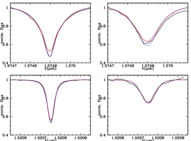
Fig. 1: Illustration of an observed Mg line (upper panels) and an Fe line (lower panels) and their respective 1D–

LTE (red) and 1D–NLTE (blue) models in the solar spectrum (Livingston & Wallace 1991). The left panels show high- resolution (R> 100000) and very high signal-to-noise ratio (S/N>800) observations, while the right panels show the same spectrum at lower resolution (R≈22000) and lower signal-to- noise ratio (S/N =100). Although the high-resolution spectra clearly highlight some modelling issues around the core of the lines, the effect is less clearly visible in the lower resolution spectrum.

they need to be strong enough to appear (and thus be measur- able) in our sample and they need to have the most reliable loggf and collisional broadening parameters so that the most accurate abundance is obtained for the observations.

2.1. Observational data

The observational data are from the SDSS IV/APOGEE2 survey (Gunn et al. 2006; Blanton et al. 2017; Majewski et al. 2017).

The data were reduced as described in Nidever et al. (2015). The selected sample corresponds to GCs members as selected by Masseron et al. (2019) and Mészáros et al. (2020), with a min- imum signal-to-noise ratio of 50 and with effective temperatures between 4000 K and 4700 K. The final observational sample comprises a total of 673 spectra of red giants across 25 globular clusters.

The effective temperatures, surface gravities, microturbulence velocities, and abundances were adopted from Masseron et al.

(2019) and Mészáros et al. (2020). However, both works noted some systematics in their Fe abundance scale compared to the literature values. Therefore, we adopt the metallicities derived by Carretta et al. (2009a,b), except for the ωCen stars, which have been disregarded. We recall that the effective temperatures were determined from photometry instead of the APOGEE data releases values, thus independently of the observed spectra to re- duce as much as possible covariances between metallicities and temperatures. Surface gravities were determined via isochrones, which have been demonstrated to be more robust against NLTE effects (Mucciarelli et al. 2015).

2.2. Model spectra

For the comparison with the data we used three sets of models:

two sets of 1D–NLTE models from two distinct codes and one set of 3D–LTE models from one 3D code.

The first set of 1D–NLTE synthetic spectra was derived with the codes TLUSTY and SYNSPEC (Hubeny & Lanz 2017).

The atom data and collisional cross-sections are the same as in Osorio et al. (2015) for Mg and in Osorio et al. (2019) for Ca. These atoms have been translated from MULTI to TLUSTY/SYNSPEC format (details in Osorio et al. 2020). The atomic and molecular line lists used will be published in Smith et al. (in prep.), except for Mg where we adopt the data from the model atom reference. For the Ca lines we adopted the parameters from Yu & Derevianko (2018) for the model atom and the atomic line list. The stellar parameters and abundances used are described in Sect. 2.1.

The second set of NLTE synthetic spectra was computed with the online synthesis tool from Kovalev et al. (2018). The radiative transfer code of that tool uses the model atoms and collisional cross-sections described in Bergemann et al. (2015) for Mg and in Bergemann et al. (2013) for Si. For the stellar parameters the online tool could not provide as many spectra as we require in a reasonable time. Therefore, we chose to compute only three representative effective temperatures for each cluster metallicity, such that Teff =4100K, 4500K, and 4700K.

Corresponding values of logg and microturbulence velocities have been interpolated from the observed data of the clusters (Sec. 2.1).

It should be noted that both 1D–NLTE sets use the same model atmospheres (MARCS Gustafsson et al. 2008), but with differences in the line lists. Nevertheless, we can assume (for close enough log gf values as is true for all the lines in this work) that the differences in the line lists cancel out when the corrections are computed consistently with the same code and the same line lists. In contrast, the two sets of 1D–NLTE models have notice- able differences regarding the implementation of the NLTE correction. The NLTE calculations performed for this work is the first application of NLTE radiative transfer calculations for several atomic species simultaneously in cool stars (Osorio et al.

2020). The calculations from Kovalev et al. (2018) are tradi- tional NLTE calculations (i.e. one atomic species is calculated at a time). The two calculations also differ in the electron and hydrogen collisional data, in particular for the levels involved in the transitions in the H band, which directly affect the statistical balance of those levels. While for electron collisional excitation we used the CCC calculations from Barklem et al. (2017) for Mg I, Bergemann et al. used the formula from Seaton (1962) taken from Zhao et al. (1998). For hydrogen collisional excitation between the low-lying levels of Mg I, the same data were used in Bergemann et al. and our works (Barklem et al. 2012);

instead, for the remaining transitions we used the free electron model from Kaulakys (1991), while in Bergemann et al. no data are reported.

Zhang et al. (2016) and Zhang et al. (2017) also made NLTE predictions for Si and Mg lines in the H band, but they did not provide the synthesis that would permit a direct comparison such as the one we discuss below. Nevertheless, their Mg model atom and collisional data were identical to the Kovalev values; their model atmospheres and statistical equilibrium code were also the same. Therefore, we expect nearly identical results to the Kovalev results presented in this work. Similarly, Zhang et al.

(2016) use comparable procedures and data to those used in Kovalev et al. (2018), although they adopt a different scaling fac-

(4)

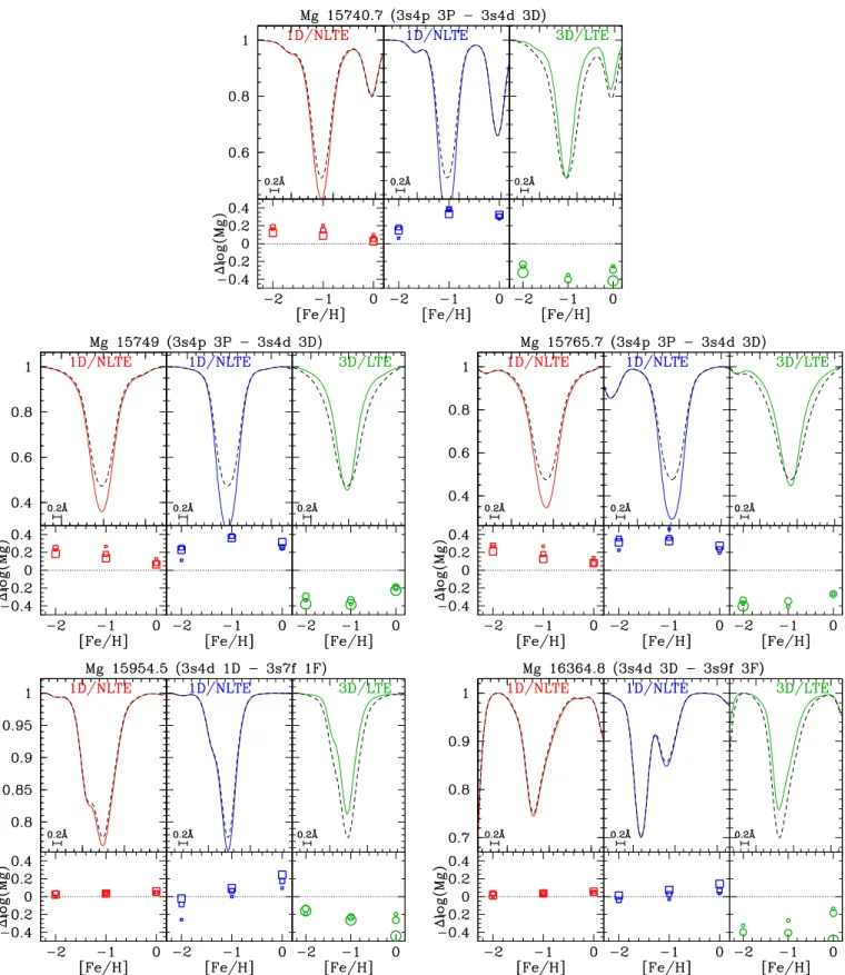
Fig. 2: Synthesis of the Mg lines used in this work. In each sub-panel the upper part shows the 1D–LTE synthesis (dashed black line), the 1D–NLTE synthesis from this work (red) and Kovalev et al. (2018) (blue), and the 3D–LTE synthesis (green) for a Teff=4500K, logg=2.5, [M/H]=−1.0 model. The lower parts display the corresponding differences in abundances of the same line between the 1D–LTE model and the NLTE or 3D models for various temperatures and metallicities (large symbols Teff=4000K, logg=1.5;

medium-size symbols Teff=4500K, logg=2.5; small symbols Teff=5000K, logg=2.5).

tor Sh=0.01 in the Drawin formula for H collisions while Ko-

valev adopts 1. Nevertheless, as we show in the following, the Si lines we are discussing here have small predicted NLTE effects, leading to negligible differences between those two works.

(5)

Fig. 3: Synthesis of Ca lines used in this work. In each sub-panel the upper part shows the 1D–LTE synthesis (dashed black line), the 1D–NLTE synthesis from this work (red), and the 3D–LTE synthesis (green) for a Teff=4500K, logg=2.5, [M/H]=−1.0 model.

The lower parts display the corresponding differences in abundances of the same line between the 1D–LTE model and the NLTE or 3D models for various temperatures and metallicities (large symbols Teff=4000K, logg=1.5; medium symbols Teff=4500K, logg=2.5; small symbols Teff=5000K, logg=2.5).

The set of 3D spectral syntheses has been taken from Ludwig et al. (in prep.) based on the 3D radiative- hydrodynamical atmosphere grid of Ludwig et al. (2009). Un- fortunately, there are only nine models corresponding to giants ({Teff,log g} = {5000,2.5},{4500,2.5},{4000,1.0}for four metallicities [M/H]=−3.0,−2.0,−1,0,0.0).

Finally, we note that although the line lists between the 3D and NLTE computations may not always be rigorously identical, the 1D–LTE mini-grids use the same corresponding line lists so that the computed abundance corrections are fully consistent.

2.3. Comparison between theoretical models

Figures 2, 3, 4, and 5 illustrate the model outputs respectively for the selected Mg, Ca, Si, and Fe lines in the H band. All of the figures compare the 3D or NLTE synthetic line profiles against 1D–

LTE synthesis for a Teff=4500K, logg=2.5, [M/H]=−1.0 model, typical of our sample stars. In these figures we note that all 1D spectra have been convolved by a macroturbulence of 3km/s with a rad-tan kernel to match the 3D simulation velocity field.

The figures also display in the lower panels the expected offset in abundance between the 3D or NLTE models and the 1D–LTE synthesis for different metallicities (−2.0,−1.0, 0.0) and different{Teff,log g}pairs ({5000,2.5}, {4500,2.5}, {4000,2.5}). The abundance offsets in these figures is equivalent to ∆log(A) = log(A)1D/LTE−log(A)NLTE,3D. We also note that the models were also degraded to the APOGEE resolution (i.e.R ≈ 22500) to ensure that theχ²minimisation process was homogeneous with the abundance analysis of the observations.

2.3.1. Mg

From Fig. 2 we can observe two main expected behaviours regarding the selected Mg lines. The first group (encompassing the 15954 and 16365Å lines) displays very small NLTE effects (for our computations and for Kovalev’s), but significant 3D effects strongly depending on metallicity. On the contrary, the second group of lines (15740, 15749, 15765Å) has large negative 3D effects but larger NLTE effects which largely enhance the line core intensity, thus leading to an overestimation of a 1D–LTE

(6)

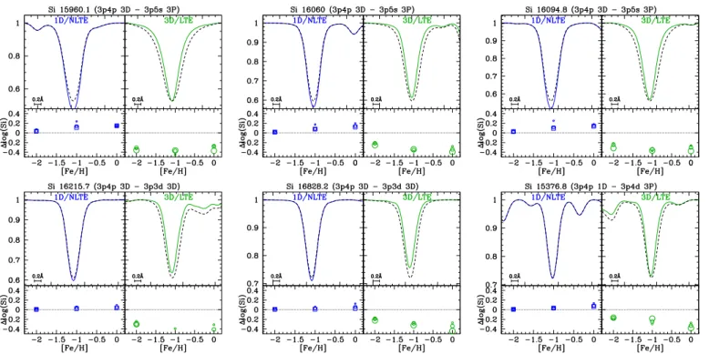
Fig. 4: Synthesis of Si lines used in this work. In each sub-panel the upper part shows the 1D–LTE synthesis (dashed black line), the 1D–NLTE synthesis from Kovalev et al. (2018) (blue), and the 3D–LTE synthesis (green) for a Teff=4500K, logg=2.5, [M/H]=−1.0 model. The lower parts display the corresponding differences in abundances of the same line between the 1D–LTE model and the NLTE or 3D models for various temperatures and metallicities (large symbols Teff=4000K, logg=1.5; medium-size symbols Teff=4500K, logg=2.5; small symbols Teff=5000K, logg=2.5).

analysis. The similarities in the second group is not surprising as the three lines belong to the same triplet. Therefore, their NLTE effects are expected to be very similar, while their relatively similar strength make them equally sensitive to 3D effects.

Furthermore, we can use Mg lines to compare NLTE predictions for two available codes and methodology. The signs of corrections generally agree between the two codes, but the amplitude may vary. The 15954Å line and to a lesser extent the 16365Å line are of particular interest because the Kovalev et al.

(2018) models predict significant corrections while our models do not. We strongly suspect that the discrepancies are due to the difference in the collisional data prescriptions. We also note that those of the 15954.5Å line show a small blend of a Ti I line on its left wing. In addition to being weak, we note that this line is included in all our line-by-line syntheses, thus taken consistently into account when applying our differential approach.

2.3.2. Ca

In contrast to Mg, none of the four Ca lines shows strong NLTE effects (Fig. 3), well in line with those reported by Osorio et al.

(2020). However, they display large 3D effects, only slightly cor- related with metallicity. Moreover, the sign and amplitude of the abundance bias is nearly identical for all lines. This is easily explained because three of them belong to the same triplet transition and the last one is the corresponding singlet transition.

2.3.3. Si

The selected Si lines show moderate NLTE and large negative 3D effects (Fig. 4). Actually, the 15376Å line does not show any NLTE effect, probably due to the fact that it is a forbidden transition. The 15960, 16060, and 16094Å lines and the 16215 and 16828Å are belonging to same triplets. Moreover, their respective strengths are similar, naturally leading to quite similar behaviour of the abundances offsets.

2.3.4. Fe

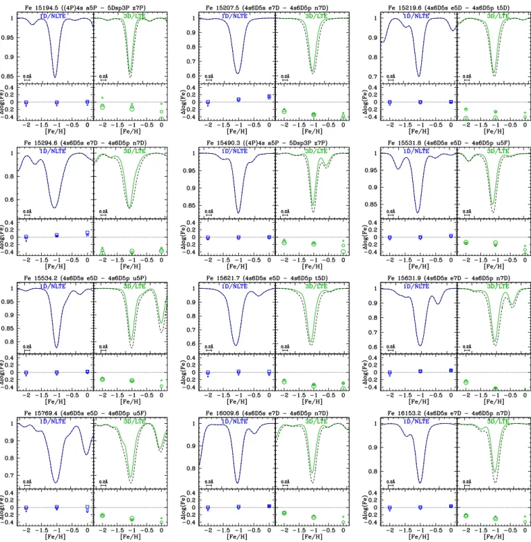
According to Kovalev’s models, the NLTE corrections for the Fe lines in H band are small (Fig. 5). Despite the large number of lines under study, it appears that the 3D corrections all show negative offsets independently of temperature and metallicity, thus suggesting that the 3D effects lead to an overestimation of the mean Fe abundance.

After examining the expected behaviours of the lines relative to the theoretical predictions of 3D and NLTE models, we can now use this information to isolate lines with a dominant NLTE or 3D effect.

3. Discussion

After reviewing the 3D and NLTE model expectations for individual lines in Sect. 2.2, we now discuss them against the data.

Although the resolution of the data does not allow a detailed line profile comparison, the effects still bias the abundance determination. In this section we use two ways to test the model predictions. The first compares the abundances obtained between two different lines. This method provides only relative estimates of

(7)

Fig. 5: Synthesis of Fe lines used in this work. In each sub-panel the upper part shows the 1D–LTE synthesis (dashed black line), the 3D–LTE synthesis (green), and for some sub-panels the 1D–NLTE synthesis from Kovalev et al. (2018) (blue) for a Teff=4500K, logg=2.5, [M/H]=−1.0 model. The lower parts display the corresponding differences in abundances of the same line between the 1D–LTE model and the 3D model for various temperatures and metallicities (large symbols Teff=4000K, logg=1.5; medium-size symbols Teff=4500K, logg=2.5; small symbols Teff=5000K, logg=2.5).

the 3D and NLTE effects, and we have applied it to the Mg and Si lines in our GCs stars sample. The second way consists in assuming that the absolute abundance of each star is known. In this regard, GCs stars offer an adequate sample as they are known to have generally homogeneous abundances of Ca and Fe, unlike Mg and Si. This method provides absolute estimates of the 3D and NLTE effects.

3.1. Probing relative 3D and NLTE effects

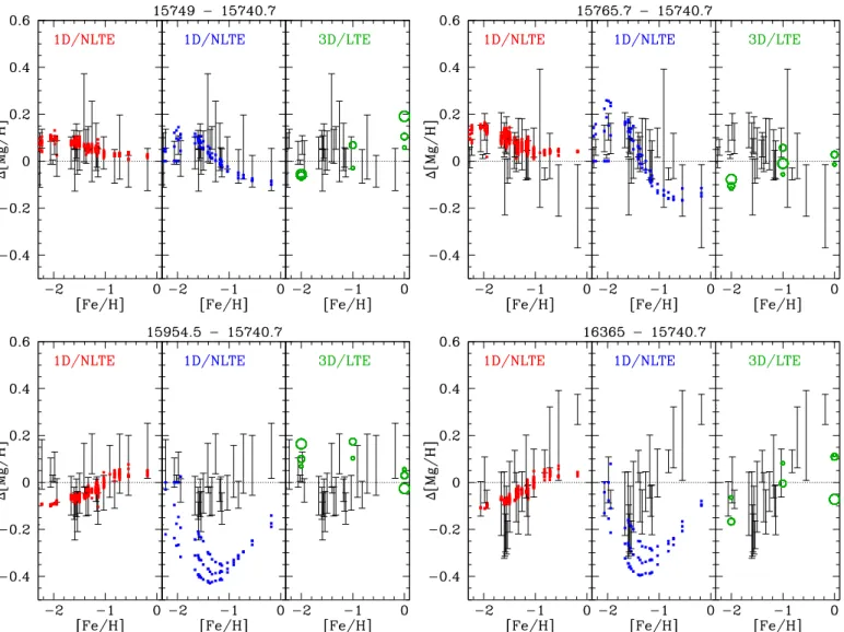
In Fig. 6 we compare the difference in abundances between two Mg lines (Sect. 2.3.1) in the data and for the 3D–LTE models and the 1D–NLTE models. In this comparison we use the 15740Å line as a common reference line between all the panels. In Sect. 2.3.1 we explain that similar 3D effects and similar NLTE effects are also expected between the reference line and the 15749 and 15765Å lines. Although the quantum properties

(8)

Fig. 6: Differences in abundance obtained between two Mg lines. The black error bars show the star-to-star median of the 1D–LTE analysis of the APOGEE data. The red squares in the left panels show the prediction obtained with the 1D–NLTE models from this work. The blue squares in the middle panels show the prediction obtained with the 1D–NLTE models of Kovalev et al. (2018). The green circles in the right panels show the prediction obtained by the 3D–LTE models of Ludwig et al. (in prep.).

of those lines are identical, we observe in Fig. 6 that the 3D and NLTE models still predict some residual behaviour probably due to the slight difference in their strengths, suggesting slightly different formation depths in the atmospheres. Both NLTE models predict a decreasing trend with increasing metallicity, which appears compatible with the data within the error bars. However, the 3D–LTE models predict a trend in the opposite direction which does not seem compatible with the data.

Concerning the two other Mg lines (15954 and 16364.8Å) the interpretation of their abundance against the reference line is more complex because these lines are expected to be 3D sensitive but not NLTE sensitive, whereas the reference line is sensitive to both. The data of 15954−15740 differences and the 16365−15740 differences do not show any offset, but do show a weak positive trend that is reproduced by our 1D–NLTE predictions but not by the Kovalev predictions. This implies either that Kovalev’s NLTE effects in a 3D hydrodynamical atmosphere environment are drastically different, or that the NLTE effects of this work cancel out between the two lines, but that the 3D effects are smaller than predicted. In this case, only self-consistent 3D–NLTE simulations could sort out the correct interpretation.

It is also interesting to note that in all panels of this figure that the predicted dispersion around the trends is relatively small even though all the stars have various stellar parameters and Mg abundances, and that we consistently took this into account in our calculations. Therefore, we conclude that the dependence of NLTE effect for those Mg lines is dominated by metallicity.

Regarding the Si lines, we observe a similar situation to that for the Mg lines (Fig. 7). There are three sets of lines: two sets of triplet transitions (15960, 16060, 16094 Å) and (16215, 16828Å), and a forbidden transition (15376 Å). We chose again one of the triplet lines as a reference line (15960Å). As for the Mg triplet lines, the observed 16060−15960 and the 16094- 15960 differential abundances are nearly null with a slight residual trend. The predicted NLTE corrections seem compatible with the data. The agreement between the data and the NLTE models appears particularly good for the 16094−15960, and a bit less in the 16060−15960 case. The differential abundance against the other lines of the other triplet (16215, 16828Å) not surprisingly gives very similar results between the two lines, and is still in very close agreement with Kovalev’s NLTE simulations.

The Kovalev predictions are in good agreement with the Si lines

(9)

Fig. 7: Differences in abundance obtained between two Si lines. The black error bars show the star-to-star median of the 1D–LTE analysis of the APOGEE data. The blue squares in the left panels show the prediction obtained with the 1D–NLTE models of Kovalev et al. (2018). The green circles in the right panels show the prediction obtained by the 3D–LTE models of Ludwig et al.

(in prep.).

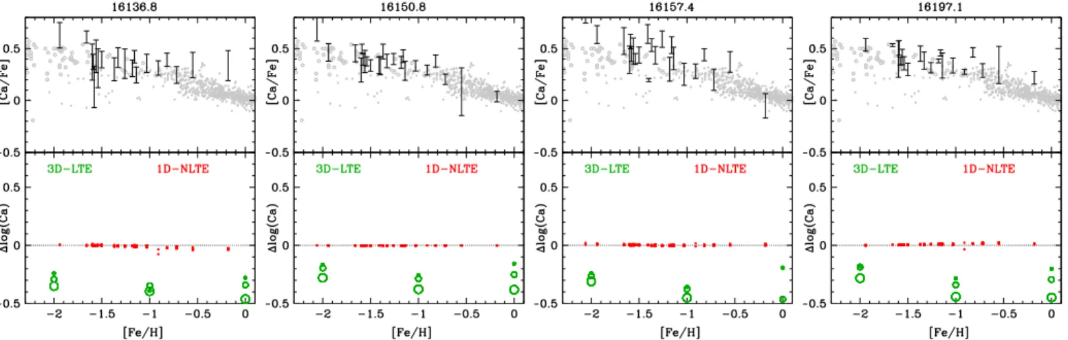
Fig. 8: Upper panels: Abundances obtained for individual Ca lines. The black error bars show the star-to-star median of the 1D–LTE analysis of the APOGEE data. The grey open circles and grey dots are literature data from respectively Roederer et al. (2014) and Bensby, T. et al. (2014) from optical dwarf spectra. Bottom panels: Corrections obtained with the 1D–NLTE models from this work (red squares) with the 3D–LTE models of Ludwig et al. (in prep.) (green circles).

abundance data while they are not in good agreement with the Mg lines abundance data. Beyond the fact that they are two distinct atoms, this could also be explained by differences in the quality and completeness of the collisional data adopted: for Mg, the Kovalev et al. (2018) code uses the Bergemann et al. (2015) model where hydrogen collisions between high excitation levels

were neglected; for Si, the Kovalev et al. (2018) code uses the model atom of Bergemann et al. (2013). This latter work used one scaling relation of the Drawin formula from Lambert (1993) to assign cross-section values for all energy levels and check it against some lines of the solar spectrum. Given that the test lines of Bergemann et al. (2013) and our lines have similar energy lev-

(10)

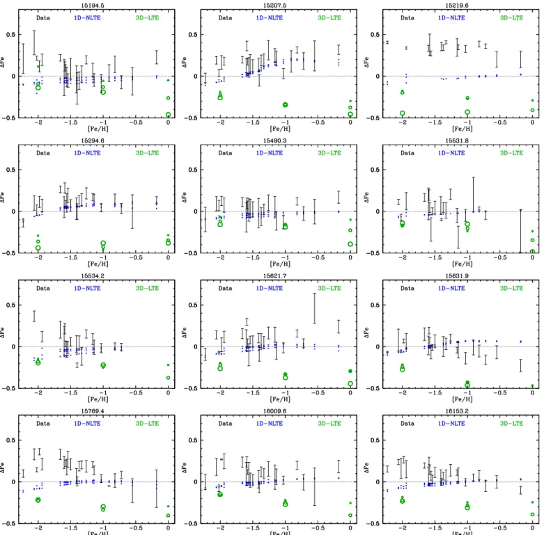
Fig. 9: Difference of abundance of Fe lines obtained from individual lines with the literature metallicity of the cluster (black error bars). The green circles show the prediction of the 3D–LTE models correction and blue squares indicate 1D–NLTE corrections from Kovalev et al. (2018).

els, this may explain why Kovalev’s NLTE predictions provide good agreement with the data. However, our study also involves the forbidden transition at 15376 Å. For that line, the data seem to disagree with Kovalev’s predictions, suggesting that the scaling relation they used to compute the Si cross-sections is not valid for all transitions. This supports the idea that the scaling relation in NLTE calculations should be avoided and, as quoted from Bergemann et al. (2013), that ‘more accurate estimates of the collision rates are desirable and, once available, will significantly improve the accuracy of the calculations’.

Regarding the 3D predictions, they show moderate amplitude with a negative dependence with metallicity, a trend which seems hardly compatible with the data. The case of the 15376Å line is of particular interest because it is a forbidden transition whose NLTE effects can be considered negligible. Therefore, the NLTE effect should only be due to the 16960Å line alone. The data suggest a v-shaped dependence against metallicity, and so do the NLTE simulations. However, there is an offset between the models and the data that might be explained by a combi- nation of the NLTE effects with the 3D effects. Therefore, the 3D–LTE spectra for the weak lines do not provide a good pre-

(11)

diction of reality, and 3D–NLTE should be more appropriate.

To verify this hypothesis a full 3D–NLTE calculation would be necessary. We finally note that the microturbulence and macroturbulence velocities in the 1D–LTE calculations could be tuned to match the 3D computations. However, while in principle these empirical parameters can be freely varied, the values we use in this work are compatible with optical studies and with APOGEE spectra standard analysis (Holtzman et al. 2015). Moreover, we argue that if this value had to be changed, it would have a drastic impact on other strong lines such as the one in Figs. 2 and 4.

3.2. Probing absolute 3D/NLTE effects

Figure 8 shows the line-by-line abundances of Ca obtained for the whole sample and is compared to the analysis of optical dwarf spectra of Roederer et al. (2014) and Bensby, T. et al.

(2014). All data sets show a global decreasing trend with increasing metallicity as expected by chemical evolution. The 3D and NLTE expected corrections are also displayed. As explained in Sect. 2.3.2, the models predictions behave very similarly between the three Ca lines, with nearly null NLTE corrections and large 3D corrections. The agreement between the optical data and the IR data in Fig. 8 suggest that the 3D corrections should not be larger than 0.1 dex overall. Another possibility would imply that optical data are affected by NLTE while IR data are affected by 3D of the same amplitude. However, 3D abundance corrections are known to be larger in dwarfs than in giants (Ludwig et al. 2008) in contradiction with the fact that the optical data are composed of dwarfs while the IR are composed of giants. Moreover, we argue that if the 3D corrections as estimated in this work were to be applied (and so for NLTE in the optical data), the chemical evolution of Ca would be affected in an unrealistic way that is incompatible with chemical evolution expectations. The line-differential work we did for Mg and Si (see Sect. 3.1) certainly supports to some extent that 3D effects on abundances are not accurate enough, or at least require that NLTE effects be simultaneously taken into account. This conclusion also corroborates theoretical predictions where 3D–LTE abundances are often worse than 1D–LTE values (Nordlander, T. et al. 2017) and is related to the NLTE-masking effect described by (Rutten & Kostik 1982).

Regarding Fe, it is striking in Fig. 9 that the data system- atically show a positive offset of ∼0.1 dex, implying that the overall Fe abundance is overestimated compared to the literature.

First of all, this bias in metallicity is not likely due to our spe- cific procedure because a similar metallicity offset is observed in other works with distinct temperature scales dealing with the APOGEE spectra (Mészáros et al. 2013; Holtzman et al. 2015;

Mészáros et al. 2015; Masseron et al. 2019). Figure 9 shows that NLTE effects do not seem to significantly affect the Fe lines in the H band. The literature reports that optical Fe lines also do not seem to be affected by NLTE. Carretta et al. (2009a,b) checked that their metallicity determined with optical Fe I and with Fe II lines are in agreement, suggesting that NLTE effects are negligible in the optical. In contrast, recent self-consistent 3D–NLTE models of one very metal-poor giant (Amarsi et al.

2016) estimate that metallicities determined from optical Fe I and Fe II lines are respectively underestimated by 0.17 and 0.08 dex. In a similar way, Mashonkina et al. (2016b) compute 1D–

NLTE corrections for many optical Fe lines in giants and provide corrections of∼0.1 dex at low metallicities. Such corrections onto the GCs metallicities of Carretta’s work may suggest that the APOGEE data provide quite accurate GC metallicities.

But before drawing any firm conclusion, these are quite coarse

estimates because the giants used in the Amarsi and Monshon- kina works are not identical to our GCs stars, and it is not clear whether the Fe lines between the studies are fully compatible. In addition, as we demonstrate in the case of Mg and Si in Sect. 3.1, all these results are strongly dependent on the current knowledge of the Fe atom and its cross-section values, which are known to be still quite poor.

Moreover, the unrealistically large predicted 3D corrections also highlight the problem of applying corrections self- consistently. An illustration of this argument can be seen when looking at the Fe lines in Fig. 9, which show the difference between the Fe abundances and the literature cluster metallicity (Carretta et al. 2009a,b). In this figure the 3D–LTE estimated corrections are overplotted and predict a negative offset, which is the opposite of the data. If we had to derive the metallicity of the 3D models with 1D models, we would certainly find a lower metallicity. By extension, we can also derive different Teffand log g (see also Chiavassa et al. 2011, where different 1D effective temperatures are derived in 3D supergiant model spectra depending on whether you use optical molecular band strength or infrared flux). In other words, the derived stellar parameters derived with 3D models may be different to the one derived in 1D, implying that 3D abundance corrections applied on 1D abundances with the same stellar parameters between 1D and 3D are not consistent; thus, a direct comparison (as in Fig. 8 and Fig. 9) may not be adequate. Actually, if we had to apply the average∼-0.3 metallicity correction from Fig. 9 in addition to the ∼-0.3 Ca corrections in Fig. 8, the net resulting corrections would be at more realistic levels. Nevertheless, we note that self-consistency is certainly an important argument for our discussion for probing absolute corrections as we do for Ca and Fe, but that does not affect our method for testing relative corrections (Sect. 3.1) where the line-differential approach ensures that the differences in stellar parameters between 1D and 3D cancel out.

4. Conclusions

In this paper we have tested the theoretical predictions of some 3D–LTE and 1D–NLTE models against a homogeneous analysis of a large sample of GC spectra from the APOGEE large spectroscopic survey. In particular, we have discussed the expected effects on the individual lines abundances of four elements (Mg, Si, Ca, and Fe). Using Mg lines, we could compare two distinct sets of models for 1D–NLTE and show that the predictions are in the same direction. Nevertheless, we observe some quantitative differences that are mainly due to the inclusion or not of good and complete collisional cross-sections, and not by the differences in the codes themselves.

The analysis of the abundance differences between several Mg lines (and similarly Si lines) allows us to also verify the impact of the 3D effects. However, some 3D–LTE predictions seem to provide a satisfactory explanation for some of the lines abundance behaviour, but most do not. Nevertheless, while waiting for more extensive 3D model grids, our work supports and gen- eralises the fact that 1D–LTE provides a better approximation than 3D–LTE, and thus that 1D–LTE calculation partially cancel out the 3D–NLTE effects (Asplund et al. 2003). We reach similar conclusions regarding Ca abundances where the 3D–LTE estimates on the Ca abundances seem too large. However, we rec- ommend strong caution when applying 3D corrections directly to 1D abundances without assuming self-consistent 3D and 1D stellar parameters.

Finally, we have checked the Fe abundances for 12 Fe lines and

(12)

show a systematic offset against the literature metallicity values.

Although more NLTE models with accurate atom data for Fe lines are crucially needed, our results may suggest that the globular clusters metallicity maybe underestimated in the optical- based literature, whereas the Fe lines of the H band offer more accurate values.

In the end our study suggests that the largest effect on abundances for late-type giants is NLTE, and that 3D is only a second- order effect that cannot be treated separately. This idea finds theoretical support in the detailed study Amarsi et al. (2016) where 1D–LTE, 1D–NLTE, 3D–LTE, and 3D–NLTE abundances of Fe lines in a few giants are compared.

The line-differential technique we develop here to probe NLTE and/or 3D models can be applied to any other elements and other data sets, and offers the great advantage of being free from knowing the abundance a priori. Nevertheless, to be valid this method still requires three things, that the stellar parameters are well constrained, that the line’s oscillator strength and collisional broadening coefficient are accurately known, and that the selected lines are relatively clean of blends.

Acknowledgements. We deeply thank H.G. Ludwig for his careful checks of the 3D spectra and thoughtful comments. We thank M. Kovalev and M. Bergemann for their great support of their NLTE online synthesis tool. We also thank A.

Amarsi for fruitful discussion about 3D/NLTE effects. T.M. acknowledges support from Spanish Ministry of Economy and Competitiveness (MINECO) under the 2015 Severo Ochoa Program SEV-2015-0548. T.M., D.A.G.H. and O.Z. also acknowledge support from the State Research Agency (AEI) of the Spanish Min- istry of Science, Innovation and Universities (MCIU) and the European Regional Development Fund (FEDER) under grant AYA2017-88254-P. Y.O, and C.A.P.

acknowledge support from the same agency under grant AYA2017-86389-P.

SzM has been supported by the János Bolyai Research Scholarship of the Hun- garian Academy of Sciences, by the Hungarian NKFI Grants K-119517 and GINOP-2.3.2-15-2016-00003 of the Hungarian National Research, Development and Innovation Office, and by the ÚNKP-19-4 New National Excellence Pro- gram of the Ministry for Innovation and Technology. This paper made use of the IAC Supercomputing facility HTCondor (http://research.cs.wisc.edu/htcondor/), partly financed by the Ministry of Economy and Competitiveness with FEDER funds, code IACA13-3E-2493. The authors also acknowledge the technical ex- pertise and assistance provided by the Spanish Supercomputing Network (Red Española de Supercomputación), as well as the computer resources used: the La- Palma Supercomputer, located at the Instituto de Astrofísica de Canarias. Fund- ing for the Sloan Digital Sky Survey IV has been provided by the Alfred P. Sloan Foundation, the U.S. Department of Energy Office of Science, and the Partici- pating Institutions. SDSS acknowledges support and resources from the Center for High-Performance Computing at the University of Utah. The SDSS web site is www.sdss.org. SDSS is managed by the Astrophysical Research Consortium for the Participating Institutions of the SDSS Collaboration including the Brazil- ian Participation Group, the Carnegie Institution for Science, Carnegie Mellon University, the Chilean Participation Group, the French Participation Group, Harvard-Smithsonian Center for Astrophysics, Instituto de Astrofísica de Ca- narias, The Johns Hopkins University, Kavli Institute for the Physics and Math- ematics of the Universe (IPMU)/University of Tokyo, the Korean Participation Group, Lawrence Berkeley National Laboratory, Leibniz Institut für Astrophysik Potsdam (AIP), Max-Planck-Institut für Astronomie (MPIA Heidelberg), Max- Planck-Institut für Astrophysik (MPA Garching), Max-Planck-Institut für Ex- traterrestrische Physik (MPE), National Astronomical Observatories of China, New Mexico State University, New York University, University of Notre Dame, Observatório Nacional/MCTI, The Ohio State University, Pennsylvania State University, Shanghai Astronomical Observatory, United Kingdom Participation Group, Universidad Nacional Autónoma de México, University of Arizona, Uni- versity of Colorado Boulder, University of Oxford, University of Portsmouth, University of Utah, University of Virginia, University of Washington, University of Wisconsin, Vanderbilt University, and Yale University.

References

Alexeeva, S., Ryabchikova, T., Mashonkina, L., & Hu, S. 2018, ApJ, 866, 153 Allende Prieto, C., Asplund, M., & Fabiani Bendicho, P. 2004, A&A, 423, 1109 Allende Prieto, C., Asplund, M., García López, R. J., & Lambert, D. L. 2002,

ApJ, 567, 544

Amarsi, A. M., Barklem, P. S., Collet, R., Grevesse, N., & Asplund, M. 2019, A&A, 624, A111

Amarsi, A. M., Lind, K., Asplund, M., Barklem, P. S., & Collet, R. 2016, MN- RAS, 463, 1518

Asplund, M., Carlsson, M., & Botnen, A. V. 2003, A&A, 399, L31

Asplund, M., Nordlund, Å., Trampedach, R., Allende Prieto, C., & Stein, R. F.

2000a, A&A, 359, 729

Asplund, M., Nordlund, Å., Trampedach, R., & Stein, R. F. 2000b, A&A, 359, Barklem, P. S., Belyaev, A. K., Spielfiedel, A., Guitou, M., & Feautrier, N. 2012,743

A&A, 541, A80

Barklem, P. S., Osorio, Y., Fursa, D. V., et al. 2017, A&A, 606, A11 Beeck, B., Collet, R., Steffen, M., et al. 2012, A&A, 539, A121 Bensby, T., Feltzing, S., & Oey, M. S. 2014, A&A, 562, A71

Bergemann, M. 2014, Analysis of Stellar Spectra with 3-D and NLTE Models, 187–205

Bergemann, M., Kudritzki, R.-P., Gazak, Z., Davies, B., & Plez, B. 2015, ApJ, 804, 113

Bergemann, M., Kudritzki, R.-P., Plez, B., et al. 2012a, ApJ, 751, 156 Bergemann, M., Kudritzki, R.-P., Würl, M., et al. 2013, ApJ, 764, 115 Bergemann, M., Lind, K., Collet, R., Magic, Z., & Asplund, M. 2012b, MNRAS,

427, 27

Bergemann, M. & Nordlander, T. 2014, NLTE Radiative Transfer in Cool Stars, 169–185

Blanton, M. R., Bershady, M. A., Abolfathi, B., et al. 2017, AJ, 154, 28 Caffau, E., Bonifacio, P., Oliva, E., et al. 2019, A&A, 622, A68 Caffau, E., Ludwig, H. G., Steffen, M., et al. 2008, A&A, 488, 1031

Carretta, E., Bragaglia, A., Gratton, R., & Lucatello, S. 2009a, A&A, 505, 139 Carretta, E., Bragaglia, A., Gratton, R. G., et al. 2009b, A&A, 505, 117 Chiavassa, A., Freytag, B., Masseron, T., & Plez, B. 2011, A&A, 535, A22 Collet, R., Asplund, M., & Trampedach, R. 2006, ApJ, 644, L121

De Silva, G. M., Freeman, K. C., Bland-Hawthorn, J., et al. 2015, MNRAS, 449, Ezzeddine, R., Merle, T., Plez, B., et al. 2018, A&A, 618, A1412604

Freytag, B., Steffen, M., Ludwig, H. G., et al. 2012, Journal of Computational Physics, 231, 919

Galsgaard, K. & Nordlund, Å. 1996, J. Geophys. Res., 101, 13445 Gilmore, G., Randich, S., Asplund, M., et al. 2012, The Messenger, 147, 25 Gunn, J. E., Siegmund, W. A., Mannery, E. J., et al. 2006, AJ, 131, 2332 Gustafsson, B., Edvardsson, B., Eriksson, K., et al. 2008, A&A, 486, 951 Hawkins, K., Masseron, T., Jofré, P., et al. 2016, A&A, 594, A43 Holtzman, J. A., Shetrone, M., Johnson, J. A., et al. 2015, AJ, 150, 148 Hubeny, I. & Lanz, T. 2017, arXiv e-prints, arXiv:1706.01859 Kaulakys, B. 1984, Journal of Physics B: Atomic, 17, 4485

Kaulakys, B. 1991, Journal of Physics B Atomic Molecular Physics, 24, L127 Klevas, J., Kuˇcinskas, A., Steffen, M., Caffau, E., & Ludwig, H. G. 2016, A&A,

586, A156

Korn, A. J., Shi, J., & Gehren, T. 2003, A&A, 407, 691

Korotin, S. A., Andrievsky, S. M., Caffau, E., Bonifacio, P., & Oliva, E. 2020, MNRAS, 496, 2462

Kovalev, M., Bergemann, M., Ting, Y.-S., & Rix, H.-W. 2019, A&A, 628, A54 Kovalev, M., M. Bergemann, Brinkmann, S., & and MPIA IT-department. 2018,

NLTE MPIA web server, [Online]. Available: http://nlte.mpia.de Max Planck Institute for Astronomy, Heidelberg.

Lambert, D. L. 1993, Physica Scripta, T47, 186

Lind, K., Amarsi, A. M., Asplund, M., et al. 2017, MNRAS, 468, 4311 Lind, K., Melendez, J., Asplund, M., Collet, R., & Magic, Z. 2013, A&A, 554,

A96

Livingston, W. & Wallace, L. 1991, An atlas of the solar spectrum in the infrared from 1850 to 9000 cm-1 (1.1 to 5.4 micrometer)

Ludwig, H. G., Caffau, E., Steffen, M., et al. 2009, Mem. Soc. Astron. Italiana, 80, 711

Ludwig, H.-G., González Hernández, J. I., Behara, N., Caffau, E., & Steffen, M. 2008, in American Institute of Physics Conference Series, Vol. 990, First Stars III, ed. B. W. O’Shea & A. Heger, 268–272

Ludwig, H.-G., Koesterke, L., & Allende Prieto, C. in prep.

Magic, Z., Collet, R., Asplund, M., et al. 2013, A&A, 557, A26

Majewski, S. R., Schiavon, R. P., Frinchaboy, P. M., et al. 2017, AJ, 154, 94 Mashonkina, L. 2014, in IAU Symposium, Vol. 298, Setting the scene for Gaia

and LAMOST, ed. S. Feltzing, G. Zhao, N. A. Walton, & P. Whitelock, 355–

Mashonkina, L., Gehren, T., Shi, J. R., Korn, A. J., & Grupp, F. 2011, A&A, 528,365 Mashonkina, L., Ludwig, H. G., Korn, A., Sitnova, T., & CaA87 ffau, E. 2013, Mem-

orie della Societa Astronomica Italiana Supplementi, 24, 120 Mashonkina, L., Sitnova, T., & Belyaev, A. K. 2017, A&A, 605, A53

Mashonkina, L. I., Belyaev, A. K., & Shi, J. R. 2016a, Astronomy Letters, 42, Mashonkina, L. I., Sitnova, T. N., & Pakhomov, Y. V. 2016b, Astronomy Letters,366

42, 606

Masseron, T., García-Hernández, D. A., Mészáros, S., et al. 2019, A&A, 622, A191

(13)

Masseron, T., Merle, T., & Hawkins, K. 2016, BACCHUS: Brussels Automatic Code for Characterizing High accUracy Spectra, Astrophysics Source Code Library

Merle, T., Thévenin, F., Pichon, B., & Bigot, L. 2011, MNRAS, 418, 863 Mészáros, S., Holtzman, J., García Pérez, A. E., et al. 2013, AJ, 146, 133 Mészáros, S., Martell, S. L., Shetrone, M., et al. 2015, AJ, 149, 153

Mészáros, S., Masseron, T., García-Hernández, D. A., et al. 2020, MNRAS, 492, Mucciarelli, A., Lapenna, E., Massari, D., et al. 2015, ApJ, 809, 1281641

Nidever, D. L., Holtzman, J. A., Allende Prieto, C., et al. 2015, AJ, 150, 173 Nissen, P. E. & Gustafsson, B. 2018, A&A Rev., 26, 6

Nordlander, T., Amarsi, A. M., Lind, K., et al. 2017, A&A, 597, A6

Nordlund, Å. & Stein, R. F. 2009, in American Institute of Physics Conference Series, ed. I. Hubeny, J. M. Stone, K. MacGregor, & K. Werner, Vol. 1171, 242–259

Osorio, Y., Allende Prieto, C., Hubeny, I., Mészáros, S., & Shetrone, M. 2020, A&A, 637, A80

Osorio, Y. & Barklem, P. S. 2016, A&A, 586, A120

Osorio, Y., Barklem, P. S., Lind, K., et al. 2015, A&A, 579, A53

Osorio, Y., Lind, K., Barklem, P. S., Allende Prieto, C., & Zatsarinny, O. 2019, A&A, 623, A103

Pereira, T. M. D., Kiselman, D., & Asplund, M. 2009, A&A, 507, 417 Randich, S., Gilmore, G., & Gaia-ESO Consortium. 2013, The Messenger, 154,

47

Roederer, I. U., Preston, G. W., Thompson, I. B., et al. 2014, AJ, 147, 136 Rutten, R. J. & Kostik, R. I. 1982, A&A, 115, 104

Sbordone, L., Bonifacio, P., Caffau, E., et al. 2010, A&A, 522, A26 Seaton, M. J. 1962, Proceedings of the Physical Society, 79, 1105

Seaton, M. J. 1962, Atomic and Molecular Processes. Edited by D. R. Bates.

Library of Congress Catalog Card Number 62-13122. Published by Academic Press, 375

Smith, V. V., Bizyaev, D., Allende Prieto, C., Cunha, K., & et .al. in prep.

Spite, M., Andrievsky, S. M., Spite, F., et al. 2012, A&A, 541, A143 Steffen, M., Prakapaviˇcius, D., Caffau, E., et al. 2015, A&A, 583, A57

ˇCerniauskas, A., Kuˇcinskas, A., Klevas, J., et al. 2018, A&A, 615, A173 Vögler, A., Shelyag, S., Schüssler, M., et al. 2005, A&A, 429, 335 Vrinceanu, D. 2005, Phys. Rev. A, 72

Yu, Y. & Derevianko, A. 2018, Atomic Data and Nuclear Data Tables, 119, 263 Zhang, J., Shi, J., Pan, K., Allende Prieto, C., & Liu, C. 2016, ApJ, 833, 137 Zhang, J., Shi, J., Pan, K., Allende Prieto, C., & Liu, C. 2017, ApJ, 835, 90 Zhao, G., Butler, K., & Gehren, T. 1998, A&A, 333, 219