Stress tests in Hungarian banking after 2008
ZOLT AN POLL AK
1pand D AVID POPPER
21Department of Finance, Corvinus University of Budapest, F}ovam ter 8, H-1093, Hungary
2ING Bank, Netherlands
Received: October 28, 2019 • Revised manuscript received: May 24, 2020 • Accepted: May 31, 2020
© 2021 The Author(s)
ABSTRACT
The 2008 crisis highlighted the importance of using stress tests in banking practice. The role of these stress tests is to identify and precisely estimate the effect of possible future changes in market conditions on capital adequacy and profitability. This paper seeks to show a possible methodology to calculate the stressed point-in-time probability of default (PD) parameter. The presented approach contains a linear autore- gressive distributed lag model to determine the connection between the logit of default rates and the relevant macroeconomic factors, and uses migration matrices to calculate PDs from the forecasted default rates. The authors illustrate the applications of this methodology using the Hungarian real credit portfolio data.
KEYWORDS
stress test, default rate modelling, migration matrix, probability of default, IRB JEL CLASSIFICATION INDICES
C13, G21
1. INTRODUCTION
The history of bank regulation at international level started in 1988 with the Basel Accord (later called as Basel I). It was a huge step forward compared to the previous period, but it had several weaknesses. The response to the criticism of Basel I, the Basel Committee proposed Basel II rules in 1999 and after numerous revisions, their implementation began in 2007. For managing credit
pCorresponding author. E-mail: pollakz90@gmail.com
risk, Basel II was specified under the first pillar of three different approaches: the standardized, the Foundation Internal Rating-Based (FIRB) and the Advanced Internal Rating-Based (AIRB) approach.
Today, the European Banking Authority (EBA) requires banks under the AIRB approach to prudently measure their risk profile and apply more accurate risk management tools. According to the new Capital Requirements Regulation (CRR), institutions“shall regularly perform a credit risk stress test to assess the effect of certain specific conditions on its total capital requirements for credit risk”(575/2013/EU, Article 177(2)). Banks should have a comprehensive stress testing framework, which is based on forecasting capital adequacy, balance sheet and the Profit and Lost (P&L) statement along different stress scenarios. As a part of this framework, credit institutions should estimate the stressed probability of default (PD) parameters that serve as important input factors for the calculation of the bank’s performance under the defined scenarios.
One of the ways to forecast PD parameters is econometric models with default rate time series as dependent variable. In this methodology, the estimated stressed default rates are transformed into stressed segment PDs using migration matrices.
The aim of this paper is to reveal connections between various macroeconomic variables and the default rate using econometric methodology on real data and estimate the stressed PD parameters based on the results. First, we present our database and the methodology, then we show the results of the default rate model. In the last part, we will transform the stressed default rates into stressed PDs.
2. INPUT DATA
2.1. Default rates
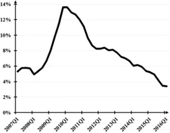
Our stress test modelling of default rates was carried out on quarterly default rate time series.
The used default definition is compliant with the CRR and applied at client level using full contamination within the loan exposures. Full contamination means that if any loan gets into default, a default event is observed for all loans of the client. The default information is added at the customer level to the database. The portfolio segment used for modelling is the micro- segment (micro-enterprises of a commercial bank’s credit portfolio). For the stress test modelling, yearly default rates were calculated for each quarter between Q1 2007 and Q1 2016.
Figure 1illustrates the default rate time series for the mentioned micro segment.
To forecast the default rates along the stress scenarios, we used different macroeconomic variables. Most of the selected macro variables are available on a quarterly basis, therefore we chose the quarterly frequency for the calculations.
Instead of modelling the default rates directly, we used the logit of them in the equations to avoid estimations outside the [0,1] interval. The logit of the default rate is calculated by the following transformation:
logit of the default rate¼log
defrate 1defrate
(1) Following the Box-Jenkins time series analysis philosophy (1976), as afirst step, we checked the stationarity of the dependent variable. The results of the unit root test Augmented Dickey- Fuller (ADF) and Phillips-Perron (PP) for logits of the default rates are as follows:
As the second row ofTable 1shows that theP-values for the logits of the default rates (not differenced) are high, so we cannot reject the null hypothesis of the unit root both in the case of ADF and PP tests. Therefore the logits are not stationary at the usually used significance levels (1%, 5% or 10%) (Table 2).
According to the final row of Table 1, the first differences are already stationary at 5%
significance level, so variables are first order integrated according to the tests. As a result, we used thefirst differences of the logits for modelling.
2.2. Explanatory macro variables
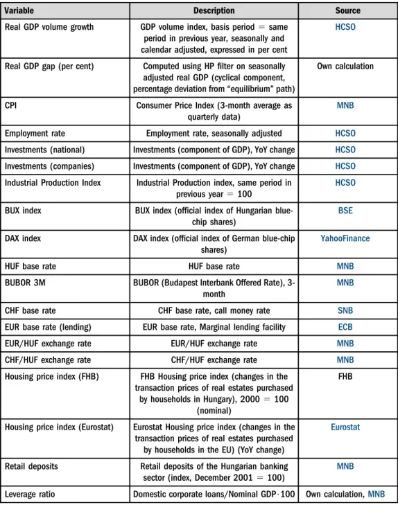
We chose the following key macroeconomic variables and used them during the stress test:
For time series analysis the explanatory variables are required to be stationary (Hamilton 1994). If stationarity is not satisfied, then the estimated models are not considered reliable, and the risk of spurious regression incurs. This is the reason for the inspection of the stationarity of the explanatory variables. ADF and PP unit root tests were carried outfirst for the level of the Fig. 1.Default rate time series
Table 1.Unit root tests of the default rate's logit
Level ADF tau ADFP-value PP tau PPP-value
Not differenced –0.0794 0.6505 –0.1324 0.6342
First difference –2.3364 0.0205 –2.4976 0.0133
Source:Authors' own calculations.
Table 2. Hungarian macroeconomic variables used for modelling (extended list)
Variable Description Source
Real GDP volume growth GDP volume index, basis period5same period in previous year, seasonally and calendar adjusted, expressed in per cent
HCSO
Real GDP gap (per cent) Computed using HPfilter on seasonally adjusted real GDP (cyclical component, percentage deviation from“equilibrium”path)
Own calculation
CPI Consumer Price Index (3-month average as
quarterly data)
MNB
Employment rate Employment rate, seasonally adjusted HCSO
Investments (national) Investments (component of GDP), YoY change HCSO Investments (companies) Investments (component of GDP), YoY change HCSO Industrial Production Index Industrial Production index, same period in
previous year5100
HCSO
BUX index BUX index (official index of Hungarian blue- chip shares)
BSE
DAX index DAX index (official index of German blue-chip shares)
YahooFinance
HUF base rate HUF base rate MNB
BUBOR 3M BUBOR (Budapest Interbank Offered Rate), 3- month
MNB
CHF base rate CHF base rate, call money rate SNB
EUR base rate (lending) EUR base rate, Marginal lending facility ECB
EUR/HUF exchange rate EUR/HUF exchange rate MNB
CHF/HUF exchange rate CHF/HUF exchange rate MNB
Housing price index (FHB) FHB Housing price index (changes in the transaction prices of real estates purchased
by households in Hungary), 20005100 (nominal)
FHB
Housing price index (Eurostat) Eurostat Housing price index (changes in the transaction prices of real estates purchased
by households in the EU) (YoY change)
Eurostat
Retail deposits Retail deposits of the Hungarian banking sector (index, December 20015100)
MNB
Leverage ratio Domestic corporate loans/Nominal GDP$100 Own calculation,MNB Notes:HCSO:Hungarian Central Statistical Office; MNB:National Bank of Hungary; BSE:Budapest Stock Exchange; FHB: a Hungarian mortgage bank; SNB:Swiss National Bank.
variables. Regarding the level, only the GDP growth rate and the GDP gap were proved to be stationary. For other explanatory variables, the differences were also examined.
We examined the results for both the first (“d”) and the yearly (“d4”) difference of the vari- ables. The choice between“d”and“d4”depends on their explanatory power on the default rates.
According to the unit root tests, all differenced variables can be regarded as stationary.
3. METHODOLOGY
The connection between the explanatory variables and the dependent variable is estimated using the linear autoregressive distributed lag model (using Maximum Likelihood estimation method).
The dependent variable is the first difference of the logit of the default rate. The explanatory variables are the previously described (already stationary transformed) macroeconomic variables and their lags of 1–4 quarter.
Furthermore, the autoregressive component of the dependent variable is also included in the regression (only the first lag is proved to be correlated with the current value). The applied autoregressive linear regression can be described by the following formula:
Yt¼atþb0_sYt−1þXk
i¼1
bi_sXt−iþ«t (2)
where
Ytdifferenced logit of the default rate of given segment in time periodt Yt−1autoregressive component
Xt−imacro variables and their lagged values (wherek54 quarters)
«t random error term
at andbicoefficients estimated by the linear regression
In the case of the dependent variable, the autocorrelation function can provide information about the number of lags to be included in the model. Generally, for the explanatory variables and their lags, the statistical significances of the estimated coefficients determine their inclusion or exclusion in the final model equation.
We performed the regression estimations using SAS 9.4 software. The stepwise procedure was an iteration process where we started by including a wider range of explanatory variables into the model. During every step, the explanatory variable with the highestP-value is omitted if thisP-value is above the pre-given threshold. If there are no more explanatory variables with P-values higher than the threshold, then the iteration is finished. An essential advantage of stepwise regression is that the order of the omitted variables can provide valuable information about the explanatory power of the variables. Thefinal model at the end of the procedure is used to carry out the estimation for the period of 2016Q2–2019Q4.
The initial (wide) circle of the explanatory variables was determined with the help of the correlation matrices. The correlation matrices help to choose which differences (either“d1”or
“d4”) and lags of the possible explanatory variables should be included in the initial regression.
If we set the p-threshold at a relatively low level, then the estimation of the coefficients will be highly reliable as they are significantly different from zero even at a strict confidence level.
However, the number of the explanatory variables will be strongly limited. The larger the threshold is, the more macro variables the estimation is based on. So, we have more possibility to capture the link between the macro environment and the default rates. The coefficient esti- mations are however less reliable as less significant variables are also kept in the model.
4. RESULTS
4.1. Model results
We started the procedure with a wider range of explanatory variables; then the statistically insignificant variables were omitted during the steps. The variables in the initial large model were chosen based on the cross-correlation matrices. The following variables were included (“D” indicates the order of difference,“L”indicates which lag is used), seeFig. 3.
After running the stepwise procedure, we got a final model.
As presented inTable 4, the p threshold of 0.2 was applied, and two of the initial explanatory variables were omitted. Real GDP growth is significant at 10%, while Leverage ratio is significant even at 5% significance level.
Table 3. The initial model
Dependent variable Logit_default rate (D1, L0)
Explanatory variables Logit_default rate (D1, L1)
Real GDP (SA) growth (D0, L0) Leverage ratio (D4, L1) Employment rate (D, L0)
BUBOR (D4, L1)
Table 4. Thefinal model
Explanatory variables Coefficient tvalue Pvalue
Intercept 0.0137 1.13 0.3270
Logit_default rate (D1, L1) 0.2543 1.82 0.1657
Real GDP (SA) growth (D0, L0) –0.0151 –3.01 0.0514*
Leverage ratio (D4, L1) 3.4005 2.48 0.0157**
R2 Adjusted R2 Number of obs. Applied p threshold
0.6884 0.6689 36 0.2
Note:***denotes that the variable is significantly different from 0 at 1% significance level;**indicates 5% and* indicates 10% significance level.
Source:Authors' own calculations (Table 3).
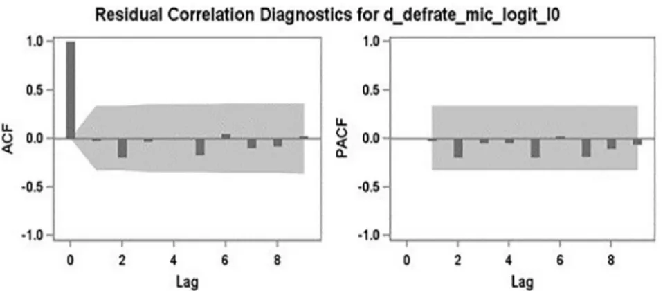
4.2. Residual correlation diagnostics
In this part, we examined whether the final model is correctly specified by checking the residuals of the estimation. In the case of a correct specification, no autocorrelation remains in the re- siduals. The autocorrelation can be checked with the graphs of ACF and PACF functions, furthermore by the Durbin-Watson test.
The ACF and PACF functions show that the residual is not strongly correlated with its own lagged values (Fig. 2). The Durbin-Watson test with its value close to 2 confirms the conclusion that the residual contains no autocorrelation (DW5 2.1584).
4.3. Model stability and impact of macro variables
Although the number of observation points is fairly small even in the full sample, the stability of the predictions has been evaluated on an out-of-time sample, as well. The model has been trained on the observations of the first 6–7 years as training sets, while the last 2–3 years have been used as test sets. Moreover, in order to quantify the additional information captured by the macroeconomic variables, the results have been compared to an AR(1) model, in which only the lagged dependent variable has been kept as regressor.Table 5summarizes the results.
Regarding the impact of the macroeconomic variables, for all specifications the final model has significantly higher explanatory power (R2) and lower prediction error (captured with Mean Squared Error) than the challenger AR(1) model. It supports that the inclusion of the macro- economic factors improves the model’s performance; therefore, the predictions’accuracy is not driven by the lagged dependent variable only.
Comparing the prediction error of the final model on the training and test sets, we found that the test errors are slightly higher than the training errors, as anticipated. For the smaller test set with only 8 observations (“Restricted model 1”) the test errors are similar to the training errors of the AR(1) model on the full sample. However, 8 observations are deemed to be quite few to be able to make general conclusions. Using the longer test sample (“Restricted model 2”), the test errors are much closer to the training errors, and they are lower than in any specification
Fig. 2.ACF and PACF functions of the residuals
of the AR(1) model. Although 12 test observations are still not numerous, this result supports that thefinal model shows good performance on separate out-of-time sample, too.
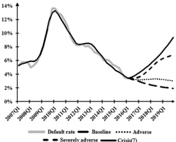
4.4. The forecasted default rates
Figure 3 plots the forecast results for the four estimated macroeconomic scenarios (baseline, adverse, severely adverse and the crisis; Crisis (7) in Fig. 3means that the crisis scenario was calculated based on the worst 7 quarters of the global financial crisis period):
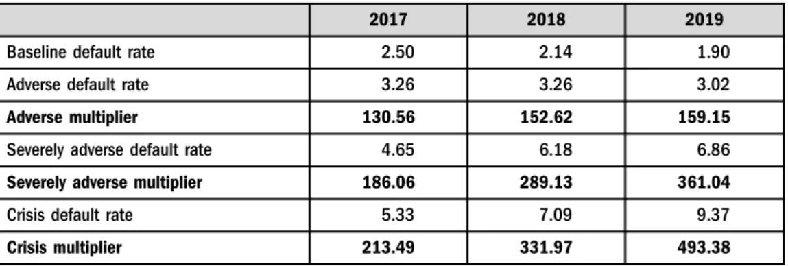
Table 6 summarizes the results numerically. Beyond the average yearly default rates (calculated as a simple average of the 4 quarters) it also presents the default multipliers. The
Fig. 3.Default rate forecast along the scenarios Table 5. Summary of the model forecasts
Model Training set Test set
Final model AR(1) model
Training Test Training Test
Adj. R2 MSE MSE Adj. R2 MSE MSE Full model 2007Q1–
2016Q1
– 0.6689 0.0038 – 0.4784 0.0057 –
Restricted model 1
2007Q1– 2014Q1
2014Q2– 2016Q1
0.7218 0.0031 0.0058 0.5242 0.0054 0.0070
Restricted model 2
2007Q1– 2013Q1
2013Q2– 2016Q1
0.7043 0.0036 0.0044 0.5025 0.0060 0.0054
Source:Authors' own calculations.
multiplier is a ratio comparing the default rate of the adverse, severely adverse and crisis sce- nario to the respective default rate of the baseline scenario. The multiplier is expressed in per cent. It tells how severe the certain scenario is, compared to the baseline forecast (Table 7).
The stress macroeconomic scenarios along with the projected paths of the macro variables are exogenous variables in terms of the model (and were provided by the Economic Research Department of a commercial bank). However, any comprehensive external macroeconomic forecast could be used for the projection, if internal predictions are not available. Regarding applicability, an important condition is that the external data source ought to be periodically updated and available for use. It produces additional risk if the stress testing activity relies on an external data source which might not be available in the future when needed for the calculations.
Table 6.Summary of the model forecasts, %
2017 2018 2019
Baseline default rate 2.50 2.14 1.90
Adverse default rate 3.26 3.26 3.02
Adverse multiplier 130.56 152.62 159.15
Severely adverse default rate 4.65 6.18 6.86
Severely adverse multiplier 186.06 289.13 361.04
Crisis default rate 5.33 7.09 9.37
Crisis multiplier 213.49 331.97 493.38
Source:Authors' own calculations.
Table 7.Base migration matrix, number of clients
C1 C2 C3 C4 C5 C6 C7 C8 D Total
C1 24 6 1 31
C2 312 641 79 2 1 5 5 6 8 1,059
C3 89 1,121 601 49 30 33 9 17 39 1,988
C4 2 121 229 37 20 10 5 11 23 458
C5 1 53 143 39 230 15 3 14 11 509
C6 18 63 26 13 10 5 5 20 160
C7 2 10 38 14 23 30 8 6 19 150
C8 15 22 18 42 28 47 63 54 289
D 1 1 531 533
Total 430 1,985 1,176 185 360 131 82 123 705 5,177
Source:Authors' own calculations.
We suggest using macroeconomic variables which are regularly forecasted by the official in- stitutions such as central banks, ECB or IMF.
5. TRANSLATING DEFAULT RATES TO PD
For further estimations within the stress testing framework, we needed segment-level1stressed PD values. That means that we had to relate the forecasted default rates with the probability of default.
This was done using migration matrices that tell us how clients’ratings change over time.
We took into account the recommendation of the European Banking Authority (EBA 2016) about the stress testing framework and migration matrices. According to this suggestion, in- stitutions need to calculate the point-in-time transition matrices, and these matrices should meet at least the following two criteria:
- The PD for each grade should calculate in line with the scenarios, and
- The probabilities of moving between grades are adjusted according to the scenarios.
Considering the above, we created the one-year observed migration matrix. The matrix shows how individual ratings changed between 2015 and 2016. As a next step, we stressed these matrices using our estimated default rate multipliers. The methodology can be described as follows:
1. We defined a common stress parameter 4that serves as a factor in which we shifted the distribution of the ratings in the matrix (4is different for every scenario).
2. We calculated the yearly default rates for the years 2016–2019 based on the observed migration matrix. These would be the“baseline”default rates.
3. We calibrated4in a way that the ratio of the stressed and the baseline default rate at the end of the forecasting horizon (2019) would be the same as the corresponding default rate multiplier estimated by the linear regressions.2
4. With these stressed migration matrices, we calculated the total exposure in every rating category for all four years.
5. Using thefixed PD of the rating categories and the total stressed exposures we can calculate the segment-level average PD for all four years.
This approach incorporates a simplification that the total number of clients remains the same over the stress testing horizon. As the number of new clients as well as the number of clients exiting the portfolio are influenced by various factors (e.g., business strategy, macro- economic environment), EBA applies a“static balance sheet assumption”when conducting its EU-wide stress testing activity. This assumption means that all assets and liabilities are fixed
1Not for the whole credit portfolio, only for the micro-enterprises segment.
2This approach answers the following question:“How much should we stress the yearly migration matrix in order to achieve the identified default rate multiplier at the end of the stress horizon, assumingfixed yearly migration pattern?”
Of course, other approaches are also possible. If the stress horizon is shorter e.g., 2 years, then the second year’s multiplier can be used for calibration. Also, if one wants to take into account the dynamics of the default rate forecast, then separate stress parameters can be calibrated for each year and scenario. However, the latter approach releases the assumption offixed yearly migration matrix, thus implicitly assumes a change of the rating migration patterns over time. These choices depend on the exact question the analyst would like to answer. The presented logic provides a general framework, which can be further tailored during the application.
during the stress horizon, as if the maturing items would be replaced by similar items. Thus, our assumption offixed portfolio size is in line with the EBA’s practice. Of course, the expected change of the portfolio can be taken into account if it is available, but it does not change the fundamental logic presented in this section.
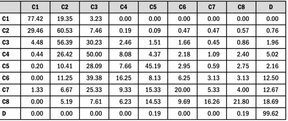
The observed one-year migration matrix (“base”migration matrix) is the following:
Expressed in per cent:
Using the migration matrix and the sum of the clients in every rating category we can easily calculate the default rates for the forecasted years that are the percentage of the non-defaulted (C1–C8) clients that migrate to the defaulted (D) rating category.
Then, we stressed the matrix by the factor4.“Stressing”means that4%of the clients in a cell is shifted to the next cell to the right, that is they migrate to a worse category. For example, if4510%
then the C1–C1 cell will be90%$77.42%569.68%, while C1–C2 cell will be90%$19.35%þ10%$ 77.42%5 25.16%. With this methodology, we can stress the whole segment depending only on one factor that can easily be calibrated to be in line with our regression estimates.
As already mentioned, the stress factor4is calibrated in a way to get the same ratio of the stressed and baseline default rates as estimated with the regressions (marked with italic in Table 6). The stressed default rates obtained using this approach might be different from the ones predicted by the model. The reason is the different baseline scenario the multiplier is applied to: in the model it corresponded to the prediction along a baseline macroeconomic scenario, while in the migration matrix-based calculation“baseline”means that the initial rating migration patterns are applied over the whole stress horizon (Table 8).
Using the fixed PDs for each grade we calculated the average segment PD. The results are summarized inTable 9.
As a summary, Fig. 4 presents the stressed segment PDs along the 4 scenarios. These PD values can be fundamentally different from the predicted default rates presented inFig. 3, as well as from the migration-based default rates shown inTable 9. The default rates inFig. 3were PiT default rates predicted by the model along the scenarios, and inTable 9they were translated into
Table 8.Base migration matrix, % of clients
C1 C2 C3 C4 C5 C6 C7 C8 D
C1 77.42 19.35 3.23 0.00 0.00 0.00 0.00 0.00 0.00
C2 29.46 60.53 7.46 0.19 0.09 0.47 0.47 0.57 0.76
C3 4.48 56.39 30.23 2.46 1.51 1.66 0.45 0.86 1.96
C4 0.44 26.42 50.00 8.08 4.37 2.18 1.09 2.40 5.02
C5 0.20 10.41 28.09 7.66 45.19 2.95 0.59 2.75 2.16
C6 0.00 11.25 39.38 16.25 8.13 6.25 3.13 3.13 12.50
C7 1.33 6.67 25.33 9.33 15.33 20.00 5.33 4.00 12.67
C8 0.00 5.19 7.61 6.23 14.53 9.69 16.26 21.80 18.69
D 0.00 0.00 0.00 0.00 0.19 0.00 0.00 0.19 99.62
Source:Authors' own calculations.
Table 9. Stressed PD results, %
Scenario 2017 2018 2019 Stress factor (4)
Baseline Default rate based on observed migration matrix
2.35 1.63 1.24
Average segment PD 4.12 3.17 2.63 Adverse Default rate based on stressed migration
matrix
3.05 2.35 1.97 20.39
Default rate multiplier 130.01 144.42 159.14 Average segment PD 5.13 4.35 3.91 Severely adverse Default rate based on stressed migration
matrix
4.99 4.58 4.47 71.41
Default rate multiplier 212.74 281.93 361.04 Average segment PD 8.02 7.90 7.86 Crisis Default rate based on stressed migration
matrix
6.03 5.93 6.11 96.16
Default rate multiplier 256.91 364.37 493.38 Average segment PD 9.62 9.95 10.18
Source:Authors' own calculations.
Fig. 4.Stressed segment PDs
expected default rates in line with the base migration matrix. In contrast, the stressed segment PDs were calculated using the calibrated long-term PDs of each rating grade.
And finally, with the help of these PDs, we can estimate the effect of the different stress scenarios to the P&L and the capital adequacy of the given financial institution.
6. CONCLUSION
We presented a possible methodology to calculate the stressed point-in-time PD parameter. This estimation is crucial for a sound stress testing, but the final methodology that a financial institution chooses has to be in line with the scope and complexity of the bank.
The regression method we applied requires a long enough time series which is not always available. Therefore alternative methods and expert-based considerations should also be taken into account. And even if econometric modelling is possible, the results should be evaluated and sometimes modified by experts who have deep knowledge of the bank’s portfolio and risk profile.
ACKNOWLEDGEMENTS
This research was supported by the Higher Education Institutional Excellence Program of the Ministry for Innovation and Technology in the framework of the“Financial and Public Services” research project (reference number: NKFIH-1163-10/2019) at Corvinus University of Budapest.
REFERENCES
Box, G. E. P.–Jenkins, G. M. (1976):Time Series Analysis: Forecasting and Control. San Francisco: Holden- Day.
Budapest Stock Exchange Statistics,https://bet.hu/.
European Banking Authority (EBA) (2016):2016 EU-Wide Stress, Test Methodological Note. 24 February 2016.
European Central Bank (ECB) Statistics,https://www.ecb.europa.eu.
Eurostat Statistics,http://ec.europa.eu/eurostat.
Hamilton, J. D. (1994):Time Series Analysis.New Jersey: Princeton University Press.
Hungarian Central Bank (MNB) Statistics,https://www.mnb.hu.
Hungarian Central Statistical Office (HCSO) Statistics,http://www.ksh.hu.
Regulation (EU) No 575/2013 of the European Parliament and of the Council of 26 June 2013 on pru- dential requirements for credit institutions and investmentfirms.
Swiss National Bank Statistics,https://www.snb.ch/en/.
YahooFinance Statistics,https://finance.yahoo.com/w.
Open Access. This is an open-access article distributed under the terms of the Creative Commons Attribution 4.0 International License (https://creativecommons.org/licenses/by/4.0/), which permits unrestricted use, distribution, and reproduction in any medium, provided the original author and source are credited, a link to the CC License is provided, and changes–if any–are indicated. (SID_1)