Application of Structured Robust Synthesis for Flexible Aircraft Flutter Suppression
Bálint Patartics , György Lipták , Tamás Luspay , Peter Seiler , Member, IEEE, Béla Takarics , Member, IEEE, and Bálint Vanek ,Member, IEEE
Abstract— This article presents a method for structured robust control design for systems with a mixture of parametric and dynamic uncertainty. The proposed method alternates between an analysis step and a synthesis step. Samples of the paramet- ric uncertainty are computed during the analysis steps, thus yielding an array of uncertain systems containing only dynamic uncertainty. The controller is then synthesized on this array of uncertain models. This synthesis step itself involves an alternation between constructing a D-scale for each of the uncertain systems and tuning a single controller for the entire collection of scaled plants. The controller tuning is performed using structured control design techniques. The proposed method is utilized to design a flutter suppression controller for a flexible aircraft.
The aircraft dynamics are described by both a high-fidelity and a reduced-order model. The design objectives for flutter suppression are to achieve robust stabilization in the presence of mixed uncertainty. The proposed structured design method yields a single, low-order, linear time-invariant (LTI) controller, which increases the flutter speed by 15%. Additional robustness analyses and high-fidelity simulations are provided to assess the controller performance.
Index Terms—µ-synthesis, flutter control, mixed uncertainty, structured synthesis, uncertain systems.
I. INTRODUCTION
T
HERE are a variety of optimal control synthesis methods available in the literature, e.g., H2and H∞methods [1], [2]. However, the practical application of these methods can be limited because they provide full-structure state-space con- trollers. Industrial applications often prefer or require con- trollers with specific structure for implementation. ExamplesManuscript received March 2, 2020; revised October 28, 2020; accepted February 21, 2021. Manuscript received in final form March 11, 2021. The research leading to these results is part of the FLiPASED project. This project has received funding from the European Union’s Horizon 2020 research and innovation programme under grant agreement No 815058. This paper was supported by the ÚNKP-20-5 New National Excellence Program of the Ministry for Innovation and Technology from the source of the National Research, Development and Innovation Fund and by the by the János Bolyai Research Scholarship of the Hungarian Academy of Sciences. Recommended by Associate Editor R. Tóth.(Corresponding author: Bálint Patartics.)
Bálint Patartics, Tamás Luspay, Béla Takarics, and Bálint Vanek are with the Institute for Computer Science and Control, H-1111 Budapest, Hungary (e-mail: patartics.balint@sztaki.hu; luspay.tamas@sztaki.hu;
takarics.bela@sztaki.hu; vanek@sztaki.hu).
György Lipták was with the Institute for Computer Science and Control, H-1111 Budapest, Hungary. He is now with AImotive, H-1025 Budapest, Hungary (e-mail: lipgyorgy@gmail.com).
Peter Seiler was with the Department of Aerospace Engineering and Mechanics, University of Minnesota, Minneapolis, MN 55455 USA. He is now with the Electrical Engineering and Computer Science Department, University of Michigan, 301 Beal Avenue Ann Arbor, MI 48109-2122, USA (email: pseiler@umich.edu).
Color versions of one or more figures in this article are available at https://doi.org/10.1109/TCST.2021.3066096.
Digital Object Identifier 10.1109/TCST.2021.3066096
include the Vega launch vehicle [3], automated landing of a civilian aircraft [4], and chemical process control [5].
The H∞ synthesis conditions can be expressed as convex constraints when the plant is nominal (no uncertainty) and the controller is allowed to be full-order and unstructured [6].
Nominal synthesis becomes nonconvex, in most cases, once structure or reduced order is imposed on the controller. One notable exception is the quadratic invariance condition [7], which allows for convex synthesis. As a consequence, most research on structured control synthesis has focused on algo- rithms that are reliable and computationally efficient on typical engineering problems (but not necessarily with proofs of global optimality).
Two notable algorithms for structured control synthesis include the H∞/H2 fixed order optimization (HIFOO) in [8]
and structured H∞ design in [9]. This article focuses on the algorithm in [9] due to its ease of use inMATLAB[10] as the hinfstructfunction. The approach has also been extended to handle multiple frequency-domain design requirements in the fixed structured design as implemented in the systune function [11].
This article builds on a previous conference paper [12]
in proposing a structured synthesis method for systems with mixed (i. e. parametric and dynamic) uncertainty. The chosen objective of the design is the minimization of the worst case gain, i. e. the maximal closed-loop H∞ norm over the set of allowable uncertainties. The algorithm utilizes an iteration in which controller synthesis is followed by analysis. This iteration continuously updates a set of “bad” samples for the parametric uncertainty. This yields a corresponding set of sampled design plants. The synthesis step itself is an iterative process, which resembles the traditional D-K iter- ation [13]. The K-step is performed as a structured design (using systune) on the collection of sampled plants. The D-step solves for the scalings associated with each sam- pled plant. In the analysis step, the worst case gain of the closed loop is calculated along with a worst case uncertainty.
A sample of parametric uncertainty is extracted from this worst case uncertainty. The subsequent synthesis step is repeated using this updated set of sampled plants.
The proposed algorithm resembles the hybrid relaxation approach in [14, Algorithm 2]. The novelty of this article lies in the control synthesis step. In particular, the hybrid relaxation given in [14] has a synthesis step that involves parameterizing a single dynamic D-scale for all uncertainty sample. It then jointly optimizes over the tunable parameters in both the scaling and controller using structured synthesis techniques [9], [10]. This approach is effective for many
1063-6536 © 2021 IEEE. Personal use is permitted, but republication/redistribution requires IEEE permission.
See https://www.ieee.org/publications/rights/index.html for more information.
problems, but the restriction to a single dynamic scaling might be conservative on certain examples, e.g., see Section IV-B in [12]. As commented in [14], it is possible to extend the hybrid relaxation to parameterize one scaling for each parametric uncertainty sample at the expense of a larger number of optimization variables.
In contrast, the approach given in this article utilizes dynamic scalings that depend on the parametric uncertainty sample. The use of parameter-dependent scalings reduces conservatism at the expense of requiring a coordinatewise D-K iteration for the synthesis. This coordinatewise iteration alter- nates between optimizing the D-scaling while holding the con- troller fixed and vice versa. This tends to be less effective than the joint scaling and controller optimization used for the syn- thesis in the hybrid relaxation approach. If the D-scales depend strongly on the value of the uncertain parameters, however, the individual D-scale construction has the advantage. This is illustrated with a concrete example in [12]. Another minor distinction is that we use a branch-and-bound implementation for the worst case gain analysis. The branch-and-bounding provides tighter analysis bounds. MATLAB implementation of the algorithm is available online [15].
To demonstrate the effectiveness of this synthesis method, and as an extension of our previous work in [12], a real-life flutter suppression control example is presented for the demon- strator aircraft of the FLEXOP project [16]. The aeroelastic flutter is an adverse interaction between the aerodynamics and the structural dynamics of the aircraft, which causes undamped oscillations that can result in catastrophic structural failure.
There are a number of active control solutions to mitigate flut- ter. The robust control framework was successfully applied in [17] and extended to the linear parameter-varying (LPV) case in [18]. Optimal blending of the inputs and outputs is utilized in [19] to maximize control effectiveness for the flutter modes and minimize the excitation of the remaining modes.
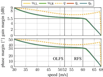
Our approach is similar to [20] with additional focus on robustness. The design model is an uncertain control-oriented model of the aircraft with both parametric and dynamic uncertainties. The control problem is decomposed into the syn- thesis of two independent single-input–single-output (SISO) controllers with the performance criteria of robust stabilization and control effort minimization. The robustness of the flutter control loop is evaluated using the high-fidelity model of the aircraft. Loop margins are computed and time-domain simulations are conducted to investigate the extension of the safe flight envelope.
The remainder of this article is laid out as follows. The syn- thesis method is described in detail by Section II. Section III presents the nonlinear high-fidelity model of the aircraft, the bottom-up modeling that results in the control-oriented model, the construction of the uncertain model, and the control design.
The analysis of the closed flutter loop is given in Section IV.
Finally, conclusions are drawn in Section V.
II. STRUCTUREDROBUSTCONTROLDESIGNALGORITHM
AGAINSTMIXEDUNCERTAINTY
The majority of this section is the restatement of the method in [12]. The mathematical formulation of the design
problem is given in Section II-A. Then, Section II-B pro- vides an overview of the algorithm. The construction of the D-scales, and the synthesis and analysis steps are elaborated in Section II-C, II-D, and II-E, respectively.
A. Problem Formulation
1) Notation : Let N ∈ CrN×cN and K ∈ CrK×cK be given matrices with rK < cN and cK < rN. Partition N such that the lower right block iscK×rK and
N =
N11 N12
N21 N22
. (1)
The lower linear fractional transformation (LFT) is
FL(N, K):=N11+N12K(I−N22K)−1N21. (2) Similarly, the upper LFT of N and∈Cr×c is defined as FU(N, ):=N22+N21(I−N11)−1N12 (3) assuming compatible dimensions. The same definitions for both the lower and upper LFTs hold ifN,K, andare linear time-invariant (LTI) systems. Finally, diag{1, 2, . . . , N} denotes the block diagonal concatenation of1,2, …, N. 2) Structured Robust Synthesis : The robust synthesis prob- lem is formulated using the feedback interconnection shown in Fig. 1. The uncertain plant P() = FU(M, ) consists of an LTI system M and structured LTI uncertainty . The objective is to design an LTI controller with fixed structure, K(κ), whereκ ∈Rnκ is a vector of tunable design parameters.
The uncertainty is assumed to be block-structured con- sisting of unit norm-bounded parametric and dynamic uncer- tainty [21], [22]. Specifically, define the following sets of parametric and dynamic uncertainties:
p: = diag
δ1Ir1, . . . , δNpIrNp δi∈R,|δi| ≤1 d: =
diag
1, . . . , Nd i LTI,||i||∞≤1 (4) where ||·||∞ denotes the H∞ norm. The dynamic blocks in d are assumed to be square. This assumption can be relaxed with only notational changes. The plant uncertainty is given as ∈ where
:=
diag
p, d p∈p andd∈d
. (5) Note that ||||∞≤1 for all ∈ . We also define a set of D-scalesDd associated with the set of dynamic uncertainties d. The set Dd consists of stable, minimum phase, and invertible LTI systems that commute with the elements of d, i.e., if Dd ∈ Dd, then Ddd =dDd, ∀d ∈ d. This set of scalings will be used in the structured robust synthesis algorithm.
Define the worst case gain of the closed loop in Fig. 1 as J(κ):=max
∈||FL(P(), K(κ))||∞. (6) This definition assumes thatFL(P(),K(κ))is robustly sta- ble, i.e., stable for all ∈ . If the closed loop is not robustly stable, then J(κ)is defined to be+∞. The synthesis
Fig. 1. Closed loop interconnection for the control design.
Fig. 2. Scaled plant used in the D-K iteration.
objective is to tune the parameters of the structured controller to minimize the closed-loop worst case gain, that is
κ=arg min
κ∈RnκJ(κ). (7)
According to our engineering experience, optimizing the worst case gain is a better performance objective than the usual robust performance [13]. If robust stability is reached, the design objective is to improve the performance without extend- ing the stability margin any further.
Structured robust synthesis is, in general, a nonconvex optimization problem. Sections II-B and II-E describe an iterative method to compute suboptimal controller parameters.
B. Overview of the Algorithm
This section introduces the proposed algorithm for comput- ing a structured controller to minimize the closed-loop worst case gain. An overview summary of the proposed approach is given in Algorithm 1. The algorithm is iterative and utilizes the sample sets for the parametric uncertainty p,s and D-scales Dd,s. The setp,s is initialized with the nominal value of the real parametric uncertainty (Step 2). These sets are updated throughout the iteration, as described further in the following.
The algorithm also expects that a controller K(κinit)is avail- able for initialization. It is further assumed that this controller robustly stabilizes the system for the dynamic uncertainty (d) and the nominal value of the parametric uncertainty (p=0).
In some problems, the open loop is robustly stable, and hence, K(κinit)=0 can be used for initialization. Otherwise, an initial robustly stabilizing controller can be computed with a related stability margin maximization algorithm.
The first key step of Algorithm 1 is to synthesize a struc- tured robust controller using an iteration (Steps 4–7) that is similar to the (unstructured, full-order) D-K iteration [13]. This
Algorithm 1 Structured Robust Synthesis
alternates between a D-step (Step 5) that computes a set of scalingsDd,sand a K-step (Step 6) that computes a structured robust controllerK(κ). This iteration terminates when ¯γddoes not decrease significantly compared to the previous iteration or when the maximum number of iterations is reached. Our specific implementation terminates the D-K inner loop if ¯γd
fails to decrease by more than 1% or the maximum number of 15 iterations is reached.
The D-step (Step 5) first constructs a set of closed loops with the structured controller K(κ), and each sample of the parametric uncertainty p ∈ p,s obtained in Step 8. Each closed-loop sample still has the remaining dynamic uncertainty d. Worst case gain analyses are performed to compute a scaling Dd∈d for each closed loop with the corresponding samplep∈p,s. Thus,Dd,shas the same number of elements as p,s. Details on this step are given in Section II-C.
The K-step (Step 6) forms a collection of scaled plants from the samples of parametric uncertainty and D-scales.
Specifically, a scaled plant is constructed for each sample (p,Dd)∈p,s×Dd,s, as shown in Fig. 2. Then,systuneis used to compute a structured controllerK(κ)to minimize the worst case gain on this collection of sampled, scaled systems.
Details on this step are provided in Section II-D.
Finally, an analysis step (Step 8) is performed on the resulting closed loop FL(P(), K(κ)). In the analysis, the entire uncertaintyis considered using a version of wcgain with additional branch-and-bounding. This generates lower and upper bounds on the worst case gain. It also computes a worst case uncertainty that achieves the lower bound. The parametric block of this worst case uncertainty is added to the sample set p,s (Step 9). Details on the analysis are given in Section II-E.
The algorithm outer-loop terminates (Step 3) if the worst case synthesis gain is within the interval of the analysis bounds, i.e.,γs ∈ [γa,γ¯a], and ¯γafails to decrease significantly (more than 1%) over the last iteration. The loop also terminates if the maximum number of iterations counts (30) is reached.
The outline of Algorithm 1 is inspired by [14, Algorithm 2].
The key difference between the two approaches is the control synthesis in Steps 4–7. Specifically, in Algorithm 1, a separate Dd ∈ Dd,s corresponds to the individual samples in p,s, instead of a common Dd. This solution reduces conservatism and decreases the number of decision variables for the struc- tured synthesis. This comes at the expense of having to use an iterative process for the controller synthesis, however. Another distinction between the two approaches is that we use branch- and-bounding for the worst case gain computation, which results in tighter bounds.
The proposed algorithm is designed to handle mixed uncer- tainty. If the system only contains dynamic uncertainty (= d), then only Steps 4–7 are performed. On the other hand, if the uncertainty is purely parametric ( = p), then the samples are LTI systems without uncertainty. In this case, Steps 4–7 are replaced by a single controller synthesis step, where we find a controller that simultaneously stabilizes all the samples and minimizes performance at the same time. This is done usinghinfstruct[9], [10].
C. Parameter-Dependent D-Scales
Let a parametric uncertainty samplep∈pand controller K(κ) be given. The corresponding closed loop T(p, κ), shown in Fig. 2, is defined as
T(p, κ):=FLFUM, p
, K(κ)
. (8)
The worst case gain for the closed loop over the remaining dynamic uncertainty is given by
maxd∈d
FUT(p, κ), d
∞. (9)
It follows from standard μ analysis results [22], [23] that an upper bound on this worst case gain over d is given by
Dmind∈Dd
γ >0
γ subject to:
Dd 0 0 √1γI
T(p, κ)
Dd−1 0 0 √1γI
∞
≤1. (10) Fig. 2 shows the sampled closed loop with D-scales and performance gain scaling. For the remainder of the derivation, the notational dependence of T on (p, κ) is dropped for
Fig. 3. Gain of the scaled system with D-scales obtained using different methods.
simplicity. Form the partitioning T =: T1
T2
where T2 has the row dimension of the error signal e. Recall that, for any complex matrix L, it follows that ¯σ(L) ≤ 1 if and only if I −L∗L 0. Here, 0 means positive semidefiniteness of the left-hand side, and L∗ is the conjugate transpose of L. This can be used to express the constraint in (10) as a (frequency-dependent) linear matrix inequality (LMI). By the Schur complement lemma, this constraint is equivalent to
⎡
⎣ γI T2(jω) T2(jω)∗
X(jω) 0 0 γI
−T(jω)∗
X(jω) 0
0 0
T(jω)
⎤
⎦0 (11)
∀ω, where X(jω):=Dd(jω)∗Dd(jω). EveryDd∈Dd has the structure diag
d1I, . . . ,dNdI , with each di as a stable, minimum-phase, invertible SISO system.
Thus, X has the structure X = diag
x1I, . . . ,xNdI , where xi = di∗di ≥ 0 for all ω. Express each xi as xi =ψ∗iψ, whereψ is a (fixed) column vector of stable, minimum phase basis functions, and i = ∗i are decision variables to be optimized.
For the subsequent synthesis step, it is advantageous to find a D-scale that does not only minimize the peak of γ but minimizes it over a broad frequency range. To illustrate this, consider Fig. 3. If we solve (10) frequency-by-frequency while allowing the D-scales to vary arbitrarily between each point, then we obtain the theoretical worst case gain lower bound.
This is the dashed blue curve in Fig. 3. If we search for a realizableDd(s)by enforcing (11) only at the frequency of the peak, thenγ (ω)we get is in general only accurate at the peak and can be far from the theoretical value at other frequencies.
See the red dashed–dotted line in Fig. 3. Using such a D-scale leaves little room for the control synthesis to improve the performance further. Therefore, it is better to enforce (11) at several frequencies at the same time. In practice, this calculation usually leads to some inaccuracy at the peak, but it provides lower γ values at the rest of the frequencies, as illustrated by the continuous yellow curve in Fig. 3.
Therefore, the constraint in (11) is enforced on a frequency grid{ωk}kN=ω1. The cost function to be minimized is turned into
γˆ +
Nω
k=1
γk (12)
where γk is the gain at ωk and ˆγ is the peak gain over all frequencies, that is
γˆ ≥γk, k=1, . . . ,Nω (13) is added to the constraints.
To ensure that xi ≥ 0 for all ω, additional Kalman–
Yakubovich–Popov (KYP) lemma constraints are added [24].
This guarantees that the solution X obtained from the opti- mization can be spectral factorized to get a stable, minimum phase scaling Dd. If ψ(jω) = Cψ jωI−Aψ−1
Bψ +Dψ, thenψ∗iψ≥0 for all ωis expressed as
(jωI−Aψ)−1Bψ I
∗ Cψ∗ Dψ∗
i
Cψ Dψ
·
(jωI−Aψ)−1Bψ I
≥0 for all ω. By the KYP lemma, this condition is equivalent to the existence of Qi =Q∗i such that
A∗ψQi+QiAψ QiBψ Bψ∗Qi 0
− Cψ∗
Dψ∗
i
Cψ Dψ
0. (14) The optimization in (10) is reformulated as the minimization of the cost function in (12) with constraints (11) for eachωk
and γk, (13) and (14). This is a convex SemiDefinite Pro- gram (SDP) in the variables ˆγ,{γk}kN=1ω ,{i}iN=1d , and{Qi}iN=1d . Finally, this optimization is solved to compute dynamic scaling
Dd for each uncertainty samplep∈p,s.
An alternative formulation of this optimization is possible in which the minimization of the cost function in (12) is decomposed into two steps. First, only the peak ˆγ is mini- mized. Second, Nω
k=1γk is minimized with γk ≤ (1+ε)γˆ, k=1, . . . ,Nω, replacing (13), whereεis a positive tolerance parameter. This approach may yield better results for some problems. Specifically, this alternative algorithm performed better on 13 of the 31 test examples (with no difference in 8 cases). However, the computation time is roughly doubled for the alternative algorithm since two optimization steps are performed.
D. Synthesis Step
The output of the D-step is a set of dynamic scalings Dd,s
each computed for a corresponding element of the parameter uncertainty setp,s. The synthesis step optimizes the controller K(κ)to minimize the worst case gain over the set of scaled, closed-loop samples. This is formulated as the following optimization:
κ∈Rminnκ
γ >0
γ subject to:
Dd 0 0 √1γI
T(p, κ)
Dd−1 0 0 √1γI
∞
≤1
∀(p,Dd)∈p,s×Dd,s. (15) This control synthesis is directly addressable using the systunecommand in MATLAB [11].
Fig. 4. Demonstrator aircraft built for the FLEXOP project.
IfK(κinit)is not robustly stabilizing for the dynamic uncer- tainty, as assumed in Algorithm 1, the D-scales are set to identity in Step 5. Under these conditions, the optimization in (15) may still yield a solution (and in fact usually does).
If there is no solution however, a different algorithm is invoked, which maximizes the stability margin of the system, thus providing a robustly stabilizing controller if possible. This algorithm is not detailed in this article for lack of space.
E. Analysis Step
The analysis step computes the upper and lower bounds on the worst case gain of the closed-loop given in (6) for a fixed controllerK(κ). This is performed using thewcgainfunction inMATLABbut modified to incorporate branch-and-bound on the parametric uncertainty. The lower boundγa is computed using a combination of a (skewed-μ) power iteration for the dynamic uncertainty blocks and a Hamiltonian-based coordi- natewise iteration on the parametric uncertainty. This returns a worst case uncertainty that achieves the lower bound. The upper bound ¯γa is computed using a frequency-gridded SDP with D-scales for the dynamic uncertainty and (D,G)-scales for the parametric uncertainty. Thus, instead of using the D-scales obtained during the controller synthesis like the algorithm in [14], we recompute the D-scales on a frequency grid for the analysis step. This is less conservative since the state-space realization of the D-scales is not required for the calculation of the worst case gain upper bound.
Branch-and-bounding of the real uncertainty is used to reduce the gap between the upper and lower bounds. Specif- ically, the real parameter uncertainty set p is described by a normalized hypercube. This hypercube is split and the upper/lower bounds are computed on each subcube. The split- ting of subcubes continues until the gap between the overall upper and lower bounds is below some relative error or a maximum number of cube splits is reached. Details on this analysis step are given in [25].
When the worst case gain upper bound ¯γa is infinite, the worst case uncertainty is chosen, which corresponds to the upper bound of the stability margin of the closed loop. This is computed using the robstabfunction inMATLAB[26].
III. FLUTTERSUPPRESSIONCONTROLDESIGN FOR THE
FLEXIBLEAIRCRAFT
The demonstrator of the FLEXOP project, shown in Fig. 4, was built specifically for flutter control experimentation [16].
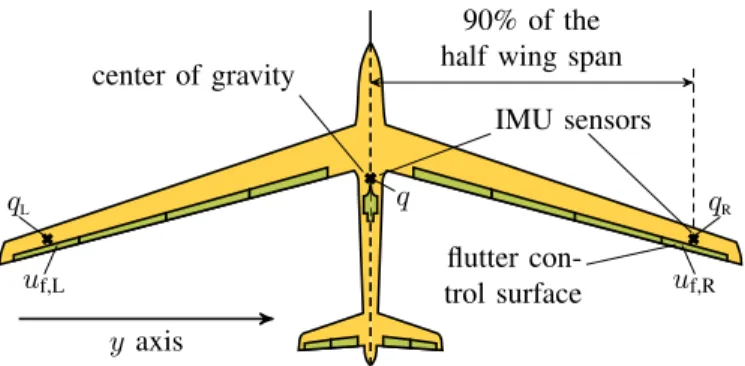
Fig. 5. Positions of the sensors and control surfaces used for the flutter suppression control. The control inputs and measurements are marked at the corresponding control surface or sensor. The signals qL, qR, and q denote angular rates along they-axis, anduf,Landuf,Rare deflection commands for the actuators.
The single-engined aircraft features a wingspan of 7 m, aspect ratio of 20, and takeoff weight between 55 and 66 kg.
This section is dedicated to the application of the structured synthesis method to the flutter suppression control design for this platform. In Section III-A, the high-fidelity model is given, which is used in the analysis of the closed loop.
The reduced-order control-oriented model is described in Section III-B. Finally, the formulation of the uncertain design model and the control problem along with the synthesis results are in Section III-C.
A. Nonlinear High-Fidelity Model of the Flexible Aircraft Each wing of the FLEXOP aircraft is equipped with four control surfaces [27] with the outermost pair dedicated to flutter suppression, as shown in Fig. 5. To actuate these, a custom-made direct-drive actuator is developed with band- width greater than the flutter frequencies. Based on system identification, the direct-drive actuator has 0.1-ms delay and transfer function
Gact(s)= 0.78s+2.74·105
s2+564.51s+2.74·105. (16) In addition to the GPS and air data probe, the aircraft features inertial measurement units (IMUs) at the center of gravity and in the wings, as shown in Fig. 5. The IMUs provide acceleration and angular rate measurements along all three body axes.
The construction of the aeroservoelastic (ASE) model is based on a subsystem approach, which involves the integra- tion of aerodynamics, structural dynamics, and flight dynam- ics [28], [29], as shown in Fig. 6. The components in Fig. 6 are developed separately and then combined to form the ASE model.
The structural dynamics are modeled by the high-fidelity finite-element method [30] and are then condensed with Guyan reduction [31]. The aerodynamics model of the air- craft is based on the vortex-lattice method (VLM) and the doublet-lattice method (DLM), and it is complemented by results from computational fluid dynamics (CFD) simulations.
The nonlinear equations of motions are derived based on a mean axes reference frame [32]. The mean axes approach
Fig. 6. ASE subsystem interconnection. Faero represents the aerodynamic forces acting on the rigid body dynamics andFexternalrepresents external, i.e., the propulsion and gravitational forces; the rest of the variables are defined in the remainder of the section.
describes the dynamics of the flexible body by a set of equa- tions that decouple the rigid body modes from the vibrational modes. The mean axes coordinates ensure that the coupling is restricted to external forcing terms only [32].
The nonlinear ASE model of the FLEXOP aircraft con- sists of 12 rigid body states, 100 states corresponding to flexible modes, and 1040 aerodynamic lag states in addition to the actuator dynamics. This model is considered as the high-fidelity model. Based on this model, the aircraft has two unstable aeroelastic modes. The symmetric flutter mode becomes unstable at 52 m/s and 50.2 rad/s, and the asymmetric mode becomes unstable at 55 m/s and 45.8 rad/s.
B. Bottom-Up Model Reduction
The high-fidelity model in III-A has over 1000 states.
Control design for such a high-dimensional model is not prac- tical; therefore, an appropriately low-order and numerically tractable control-oriented model is required [17]. Because the size of this model poses considerable difficulty to the LPV reduction techniques [33], [34], the “bottom-up” modeling approach in [35] and [30] is applied in this article. The key idea is to reduce the components of the system in Fig. 6 separately. Since the structural and aerodynamics subsystems have a simpler structure than the combined ASE model, it is possible to simplify them using more straightforward reduction techniques. This approach leads to a sufficiently low-order ASE control-oriented model.
The outermost control surface pair is used for flutter sup- pression, as shown in Fig. 5. The actuating signal is the control surface deflection command received by the actuator denoted asuf,Landuf,R for the left and right wings, respectively. The sensors used for flutter control are three IMUs: one in the center of gravity and two at the 90% of the half wingspan on each wing. Only the angular rate measurements along the y-axis of the three IMUs are used (see Fig. 5). The signals of the IMUs on the left and right wings are denoted by qL and qR, respectively, while q denotes the pitch rate in the center of gravity. Only these inputs and outputs are considered in the reduction.
The frequency range of interest where the control-oriented model is expected to provide a good approximation of the high-fidelity model is [0,100] rad/s; 100 rad/s is roughly twice the flutter frequencies 50.2 and 45.8 rad/s, which ensures the accurate representation of the flutter behavior. It is possible to retain the accuracy of the control-oriented model over a wider frequency range at the expense of additional dynamics.
The objective of the reduction is to decrease the number of states of the subsystems in Fig. 6 while maintaining an acceptably low ν-gap between the high-fidelity and the control-oriented model in the frequency range of interest ([0,100] rad/s). The ν-gap metric δν(·,·) is used since it considers the feedback control objective. It assumes values between zero (for identical systems) and one. If a feedback controller stabilizes the system P1(s)with stability marginε, then it also stabilizes P2(s)if δν(P1(s), P2(s)) < ε. A plant at a distance greater than ε from P1, on the other hand, will in general not be stabilized by the same controller [36]. The ν-gap between P1(s)and P2(s)at the fixed frequencyωis
δν(P1(jω),P2(jω))=σ¯ I+P2(jω)P2∗(jω)−1/2
· (P1(jω)−P2(jω)) I+P1∗(jω)P1(jω)−1/2
2 (17) where ¯σ[·] denotes the largest singular value.
The aerodynamic lag terms assume the state-space form
˙
xaero = 2VTAS
¯
c Alagxaero+Blag
⎡
⎣x˙rigid
˙
˙η δcs
⎤
⎦
yaero =Clagxaero (18)
whereVTASis the true airspeed (TAS), ¯cis the reference chord, xrigid is the rigid body state, η is the state of the structural dynamics, and δcs is the control surface deflection.
Balancing transformation is applied for the aerodynamics model given byAlag,Blag, andClagin (18). The order reduction is achieved by residualizing the states with the smallest Hankel singular values. Keeping two lag states results in acceptable accuracy. Coefficient CQ3η1 for the modal generalized force (see Chapter 7 of [32] for more details) affecting the symmet- ric flutter mode and coefficient Clp affecting the asymmetric flutter mode of the control-oriented model was scaled by 0.65 and 1.6, respectively. By this heuristic modification, the resulting control-oriented model matches the flutter speeds and frequencies of the high-fidelity model better. The effect of this modification on the rest of the dynamics is negligible.
The structural dynamics of the aircraft are of the form Mη¨+Cη˙+Kη=Fmodal (19) whereM,C, andKare the modal mass, damping, and stiffness matrices, respectively, and Fmodal is the external excitation in modal coordinates. The structural dynamics model is an LTI system; therefore, state truncation is applied. Along with the first six structural modes, modes 19, 20, and 21 are retained since their removal results in a large increase in theν- gap between the high-fidelity and the control-oriented model.
In this way, the 100th order structural dynamics model is reduced to 18 states. It is assumed that the structural dynamics
Fig. 7. ν-gap values as a function of frequency between the high-fidelity and the control-oriented model for the inputs and outputs used for the flutter suppression control design.
Fig. 8. Pole migration of the control-oriented and high-fidelity models.
model has parametric uncertainty. Specifically, the first six modes of the control-oriented model have ±1% uncertainty in the natural frequency and ±10% in their damping.
The resulting bottom-up control-oriented model has 56 states that consist of 12 rigid body states, 18 structural dynamics states, two aerodynamic lag states, and 24 actuator dynamics states. The design model is obtained by trimming and linearizing this model for straight and level flight at 36 equidistant points of the airspeed in the interval [30,65] m/s and for each combination of the perturbed parameters in the structural dynamics. The ν-gap between the high-fidelity and the control-oriented model for different airspeed values and the nominal structural dynamics is shown in Fig. 7. Theν-gap is calculated for the inputs and outputs used for flutter control (see Fig. 5).
The pole migration of the high-fidelity and the control-oriented model is compared in Fig. 8. The full-order model predicts flutter at 52 and 55 m/s at frequencies of 50.2 and 45.8 rad/s, respectively. In comparison, flutter occurs in the control-oriented model at 52 and 56.5 m/s at 50.3 and 46 rad/s, respectively. The flutter speed and frequency accuracy of the control-oriented model is deemed sufficient for control design.
C. Flutter Suppression Control Synthesis
In this section, the flutter suppression control design for the flexible aircraft in Section III-A is discussed. First, two uncertain SISO models are obtained from the reduced-order
Fig. 9. Structure of the control loop using two SISO controllers to stabilize the symmetric and asymmetric flutter modes separately.
control-oriented model detailed in Section III-B. Then, the performance specification used for the optimal control design is described. Finally, the results of the synthesis method in Section II are given.
1) Design Model : Selecting the control surfaces and sensor signals as described in Section III-B (and in Fig. 5) allows us to separate the symmetric and asymmetric flutter modes of the aircraft using the combination of these variables shown in Fig. 9. Two SISO systems are obtained this way: ˜Gsym(s)and G˜asym(s). The input and output of ˜Gsym(s)areuf,L+uf,Rand qL+qR−2q, respectively. The states consist of w (vertical velocity),q (pitch rate), the modal coordinates that correspond to the symmetric deformations, the lag states, and the actuator states. For ˜Gasym(s), the input and output are uf,L−uf,R and qL−qR, respectively. The states arev (horizontal velocity), p (roll rate),r (yaw rate), the modal coordinates corresponding to the asymmetric deformations, and lag and actuator states.
Both parametric and dynamic uncertainty are introduced using ˜Gsym(s) and ˜Gasym(s). As the result of the model reduction technique in Section III-B, the state-space matrices of these systems are given on a parameter grid. The grid consists of 36 equidistant points of the TAS between 30 and 65 m/s, five points of the natural frequency in the structural dynamics between±1% of the nominal value, and five points of the damping in the structural dynamics between ±10%
of the nominal value. These two arrays of LTI systems are used to introduce parametric uncertainty in the system. The dependence of the dynamics on the airspeed is expressed via the uncertain parameter δV. The uncertainty of the nat- ural frequency and the damping in the structural dynamics correspond to uncertain parameters δω0 and δξ, respectively.
The parameters are normalized uncertainties, i.e., |δV| ≤ 1, δω0≤1, and δξ≤1. Least-squares fitting is performed to obtain the uncertain state-space matrices of the form
Aδ = A0+A1δV+A2δV2 +A3δω0+A4δω20+A5δξ
Bδ = B0+B1δV +B2δ2V
Cδ =C0+C1δV +C2δ2V
Dδ =0
where{Ai}4i=0,{Bi}2i=0, and{Ci}2i=0are constant matrices. The elements of Aδ, Bδ, andCδ are assumed to be a second-order polynomial inδV based on Chapter 5 in [37]. OnlyAδdepends onδω0andδξ since the perturbation in the damping and natural
Fig. 10. Uncertain plant interconnection with the dynamic uncertaintyd(s) and Aδ,Bδ, andCδmatrices depending on the parametric uncertainty.
Fig. 11. Bode magnitude plot of the dynamic uncertainty weights.
frequency influences the position of the poles. Also, this form ofAδ,Bδ, andCδ provides low error when compared to ˜Gasym
and ˜Gsym in the parameter grid points.
Dynamic uncertainty is added to account for the model reduction in Section III-B. As shown in Fig. 10, input mul- tiplicative uncertainty structure is chosen, i.e., both uncertain SISO plants have the form
G(s)=Cδ(s I−Aδ)−1Bδ(1+Wd(s)d(s)) (20) whered(s)is the stable SISO uncertainty block for which
||d(s)||∞ ≤ 1, Wd(s) is the weight of the uncertainty, and the subscripts “sym” and “asym” are omitted. The weight is obtained by comparing the singular values of the system Cδ(s I −Aδ)−1Bδ to the high-fidelity model, which results in
Wd,sym(s)= 33.31(s+111.7)s2+49.17s+2195 (s+409.5)s2+97.17s+198900 Wd,asym(s)= 55.703(s+100)(s+40)2
(s+400) s2+350s+25000.
The Bode magnitude plot of both of the weights is shown in Fig. 11. These weighting functions serve to add moderate uncertainty at low frequencies and significant uncertainty at high frequencies. The level of uncertainty starts to rise considerably at the flutter frequencies and it is above one (100%) after 100 rad/s. This is in accordance with theν-gap results of the model reduction in Section III-B (see Fig. 7).
The resulting uncertain systems are written in the LFT form as
G(s)=FU(N(s), (s)) (21) where(s)is the structured uncertainty block containing the three uncertain parameters δV, δω0, and δξ and the dynamic uncertainty blockd(s). Therefore, forGsym(s)andGasym(s), respectively, the uncertainty sets sym andasym are defined as in (5) with
p,sym = diag
δVI51, δω0I45, δξI7
p,asym =
diag
δVI49, δω0I45, δξI7
d,sym =
d,sym
d,asym =
d,asym
.
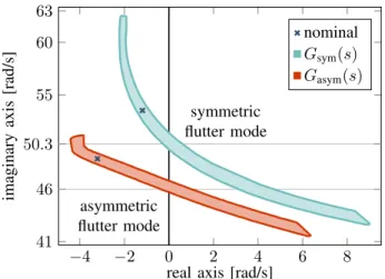
Fig. 12. Domain of the migration of the flutter mode poles due to the parametric uncertainty.
Fig. 13. Bode magnitude plot of the nominal value and random samples of the uncertain systemsGsym(s)andGasym(s).
The number of repetitions is especially high for δV and δω0. The LFR-toolbox for MATLAB could be used to reduce the size of (s) [38], but since the control synthesis method in Section II samples the uncertain parameters, this is unnecessary.
The poles ofGsym(s)andGasym(s)migrate with the change of the uncertain parameters. The domain of migration of the flutter modes is shown in Fig. 12. The introduction of δω0
and δξ in Gsym(s) and Gasym(s) captures the uncertainty in frequency and damping ratio in addition to the variation with airspeed. Note that the nominal systems are stable. The gain of the two systems changes due to both types of uncertainty.
In Fig. 13, the Bode magnitude plot of the nominal systems is depicted along with random samples. In the frequency range below the flutter frequencies, only a moderate variation is observable, while for frequencies above 100 rad/s, the gain of the systems is highly uncertain. Since the nominal systems are stable, the gain at the flutter frequencies are finite for both Gsym(s) and Gasym(s). For some values of the uncertainty, the gain of these systems is significantly higher or even unbounded.
2) Performance Specification : The purpose of the flutter controller is to robustly stabilize the undamped vibrations of
Fig. 14. Generalized plant interconnection.
the aircraft. There are further considerations to be considered.
The effect of the flutter controller on the rigid body behavior of the aircraft ought to be minimal so that the flutter controller does not interfere with the baseline controller governing the rigid body motion of the aircraft. The controller is to be imple- mented on an embedded computer whose sampling frequency is 200 Hz. Beyond this constraint, the bandwidth of the flutter controller must not breach the limitation posed by the actuator.
Also, the closed loop must remain stable even in the presence of 15-ms output delay introduced by the autopilot hardware.
The generalized plant interconnection in Fig. 14 incorpo- rates all the requirements above for bothGsym(s)andGasym(s). The 15-ms delay is represented byτ(s)that is the fourth-order Padé approximation of e−0.015s. The controller is augmented with the filter
F(s)= 1.6·105
s2+560s+1.6·105 (22) to ensure appropriate bandwidth. In this way, the sampling constraint is met and the excitation of high-frequency dynam- ics is avoided. The Bode magnitude plot of F(s)along with the performance constraints is shown in Fig. 15.
The task of robust stabilization is expressed as sensitivity minimization. The sensitivity function of both closed loops is S(s)=(1/1+τ(s)G(s)K(s)F(s)). For any stable SISO loop, the minimal distance between the open-loop Nyquist curve and the −1 point is the inverse of the peak of|S(jω)|, i.e., (1/maxω|S(jω)|)= (1/||S(s)||∞) [1]. It is also known that the gain margin of the loop is at least(||S(s)||∞/||S(s)||∞−1) and the phase margin is at least 2 sin−1((1/2||S(s)||∞)) [1].
Therefore, we want to achieve ||S(s)||∞ ≤ 2 since this provides at least 6-dB gain margin and close to 30◦ phase margin. To that end, the weight of the tracking error (i.e., the sensitivity function) is chosen as We(s)=(1/2). To limit actuator effort, the weight of the control input is Wu(s) = (1/10◦)=5.78.
3) Synthesis : The structure of the flutter suppression controller is shown in Fig. 16. The SISO controllers are parameterized as general second- and fourth-order transfer functions, that is
Kasym(s)= κ1s2+κ2s+κ3
s2+κ4s+κ5
(23) Ksym(s)= κ6s4+κ7s3+κ8s2+κ9s+κ10
s4+κ11s3+κ12s2+κ13s+κ14
(24) where{κk}14k=1are tunable design parameters. For the synthesis of Kasym(s), a frequency grid of 30 points and five basis functions were used. For Ksym(s), the number of frequency points and basis functions is 90 and 9, respectively.
Fig. 15. Bode magnitude plot ofF(s)and the performance constraints. The actuator dynamicsGact(s)are given in (16).
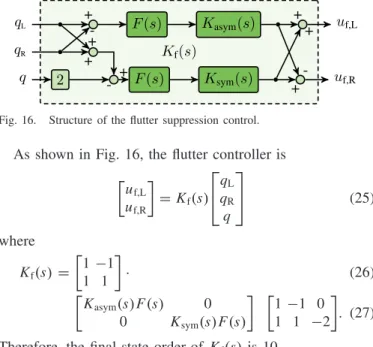
Fig. 16. Structure of the flutter suppression control.
As shown in Fig. 16, the flutter controller is uf,L
uf,R
=Kf(s)
⎡
⎣qL
qR
q
⎤
⎦ (25)
where Kf(s)=
1−1 1 1
· (26)
Kasym(s)F(s) 0 0 Ksym(s)F(s)
1−1 0 1 1 −2
. (27) Therefore, the final state order of Kf(s)is 10.
The two SISO loops are tuned separately. As the result of the synthesis, the tunable components of Kf(s)are
Kasym(s)= 0.0106s2+0.5476s+53.6039 s2+40.4171s+904.595 Ksym(s)
=0.0126s4+3.7765s3+1479.85s2+48443.9s+444523 s4+114.354s3+59809.2s2+538987s+1.4737·106 . It takes ten iterations (i.e., ten samples of p,asym) to obtain Kasym(s) and nine iterations (nine samples of p,sym) are required for Ksym(s).1 The singular values of the flutter con- troller are shown in Fig. 17. The controller has enough control authority at the flutter frequencies, and it is sufficiently rolled off at the sampling frequency. The performance of Kf(s) is analyzed in closed loop with the high-fidelity model linearized at certain speed values in Section IV.
IV. EVALUATION OF THEFLUTTERCONTROLLERUSING THENONLINEARHIGH-FIDELITYMODEL
This section details the evaluation of the flutter controller described in Section III. First, the baseline control architecture is presented that governs the rigid body motion of the aircraft.
1The computation takes approximately 3 h on a computer that runs Ubuntu 16.04 LTS and features an eight-core 2.1-GHz Intel Xenon CPU with 20 GB RAM. The algorithm is run onMATLABR2016b making use of the Parallel Computing Toolbox.
Fig. 17. Singular values of the flutter controller along with the frequency-domain constraints.
Fig. 18. Control surface configuration of the baseline control architecture.
The control inputs are marked at the corresponding control surface.
Then, the stability, performance, and robustness analysis are described with the baseline and flutter suppression control loops closed. These results are also contrasted with a design based on a single D-scale instead of the D-K iteration. Finally, two time-domain simulations are conducted to confirm the frequency-domain results. All tests are performed using the linearized versions of the nonlinear high-fidelity model in Section III-A.
A. Baseline Control Architecture
The rigid body motion of this aircraft is described by a standard nonlinear six-degree-of-freedom flight mechanics model (e.g., [39]) in terms of translational velocitiesu,v, and w and angular velocities p (roll),q (pitch), and r (yaw) in the body-fixed frame. Orientation in the earth-fixed reference frame is described in terms of Euler angles (bank), (pitch), and (heading). The angles between the body-fixed frame and the wind axes are angle of attack α and side-slip angleβ. The flight path is described with respect to the earth by the path angleγ and the course angleχ.
For the actuation of the rigid body motion, four ruddervators on the V-tail of the aircraft are used, two on the left (urv,L1, urv,L2) and two on the right side (urv,R1, urv,R2), as shown in Fig. 18. These ruddervators are combining the functionalities of classical rudders and elevators. The symmetric deflections of the ruddervator correspond to classical elevator deflections, whereas asymmetric deflections exhibit rudder deflections.
In addition, four control surfaces are available on each wing.
As discussed in Section III, the outermost pair (uf,L, uf,R) is used for flutter control, whereas the innermost pair is used as high lift devices during takeoff and landing. The remaining two
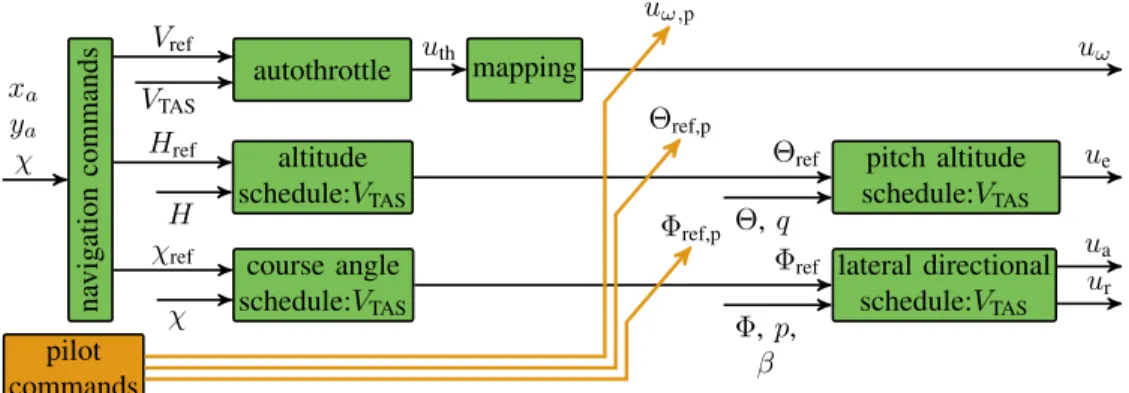
Fig. 19. Control architecture for fully automated flight and augmented flight (indicated in orange).
TABLE I
SUMMARY OF THECONTROLLOOPS OF THEFLEXOP BASELINEFLIGHT CONTROLSYSTEMWITH THEINNERLOOPFUNCTIONS(FIRSTPART)
ANDAUTOPILOTFUNCTIONS(SECONDPART)
pairs (ua,L2,ua,R2,ua,L3, andua,R3) are utilized in the baseline control law as ailerons to actuate the roll motion of the aircraft.
The structure of the baseline controller is a classical cas- caded setup shown in Fig. 19. The lateral-directional control problem is necessarily multivariable and requires the coor- dinated use of aileron command ua and rudder command ur. The innermost loop features roll-attitude () tracking, roll-damping augmentation via the roll rate (p), and coor- dinated turn capabilities, i.e., turns without side slip, via feedback of the side-slip angle (β). The outer loop establishes control of the course angle (χ). All controllers are scheduled with velocity to increase the performance over the velocity range. Within the fully automated flight mode, the reference signals for the velocity (Vref), altitude (Href), and course angle (χref) are provided by a dedicated navigation algorithm. It uses the GPS longitudinal and lateral position of the aircraft (xa
and ya) as well as the current course angle (χ) to provide the commands. More details on the algorithm can be found in [40].
Structurewise, the control loops use scheduled elements of proportional–integral–derivative (PID) controllers with addi- tional roll-off filters in the inner loops to ensure that no aeroelastic mode is excited by the baseline controller.
A scheduling in dependence of the TAS VTAS is used to ensure an adequate performance over the velocity range from 32 to 70 m/s. For the scheduling, a first- or second-order polynomial inVTASis applied. The free parameters are directly included in a structured controller optimization problem.
A comprehensive summary of the used controller structures for each cascaded loop is provided in Table I, including
Fig. 20. Change of pole trajectories due to the flutter and baseline controller.
the channel description in the controller architecture and the implemented scheduling.
Note that these controller outputsue,ua, andur defer from the actual surface inputs to ease the control design task. Thus, they need to be transformed to physical actuator commands via an adequate control allocation. The commands to the actuators of the two aileron pairs are determined by
ua,L2 =ua,L3=0.5ua
ua,R2=ua,R3= −0.5ua
to generate the required differential aileron deflections for roll motion control. For the ruddervators, superposition of the elevator command ue and the rudder commandur is applied by
urv,L1 =urv,L2=ue+0.5ur urv,R1 =urv,R2=ue−0.5ur.
Thus, symmetric deflections on the left and right of the rudder- vators correspond to elevator commands, whereas differential deflections establish rudder commands. The free parameters of the control laws are tuned to satisfy certain performance and robustness criteria as explained in [40].
B. Closed-Loop Stability and Performance Evaluation The pole trajectories of the closed loop (with both the flutter and baseline controller) are shown in Fig. 20.
The damping of both flutter modes is increased significantly.
The asymmetric flutter mode is stabilized up to 70 m/s,