MŰHELYTANULMÁNYOK DISCUSSION PAPERS
INSTITUTE OF ECONOMICS, CENTRE FOR ECONOMIC AND REGIONAL STUDIES, HUNGARIAN ACADEMY OF SCIENCES - BUDAPEST, 2018
MT-DP – 2018/3
Multidimensional global games and some applications
DZSAMILA VONNÁK
Discussion papers MT-DP – 2018/3
Institute of Economics, Centre for Economic and Regional Studies, Hungarian Academy of Sciences
KTI/IE Discussion Papers are circulated to promote discussion and provoque comments.
Any references to discussion papers should clearly state that the paper is preliminary.
Materials published in this series may subject to further publication.
Multidimensional global games and some applications
Author:
Dzsamila Vonnák junior research fellow Institute of Economics
Centre for Economic and Regional Studies, Hungarian Academy of Sciences E-mail: vonnak.dzsamila@krtk.mta.hu
January 2018
3
Multidimensional global games and some applications
Dzsamila Vonnák
Abstract
I extend the standard global games framework by introducing an addition target on which agents can coordinate on. I compare this multidimensional case to the standard global games problem. Furthermore, I investigate the effects of consolidating the multiple targets. I find that introducing an additional option generates a negative strategic correlation between the options and thus weakens the coordination. However, unifying the options eliminates the endogenous correlation and thus restores the coordination. I also show two potential applications to be modeled by these kinds of games.
Keywords: global games, coordination
JEL: C72, D84
Acknowledgement
I am grateful to Péter Kondor for his guidance on my research. I would like to thank Roland Beck, Andrea Canidio, Gabriel Desgranges, Miklós Koren, Marion Oury and Ádám Szeidl for their valuable comments. I gratefully acknowledge financial assistance from the Hungarian Academy of Sciences Momentum Grant 'Firms, Strategy and Performance'.
All errors and omissions are mine.
Több dimenziós globális játékok és néhány alkalmazásuk
Vonnák Dzsamila
Összefoglaló
A tanulmányban kiterjesztem a sztenderd globális játékok keretét egy újabb koordinációs célponttal. Ezt a többdimenziós esetet összehasonlítom a sztenderd globális játék modellel.
Ezen kívül azt is megvizsgálom, hogy milyen hatása van a koordinációs célpontok egyesítésének. Azt találom, hogy egy újabb koordinációs opció megjelenése negatív stratégiakorrelációt generál a célpontok között és így gyengíti a koordinációt. A célpontok egyesítése viszont kiküszöböli ezt az endogén korrelációt és így visszaállítja a koordinációt.
A tanulmányban két olyan alkalmazást is bemutatok, amelyek modellezésére alkalmas lehet ez a játékelméleti keret.
Tárgyszavak: globális játékok, koordináció
JEL kód: C72, D84
Multidimensional global games and some applications
∗Dzsamila Vonn´ak† January 25, 2018
Abstract
I extend the standard global games framework by introducing an addition target on which agents can coordinate on. I compare this multidimensional case to the standard global games problem. Furthermore, I investigate the effects of consolidating the mul- tiple targets. I find that introducing an additional option generates a negative strategic correlation between the options and thus weakens the coordination. However, unifying the options eliminates the endogenous correlation and thus restores the coordination.
I also show two potential applications to be modeled by these kinds of games.
JEL Classification: C72, D84 Keywords: global games, coordination.
∗I am grateful to P´eter Kondor for his guidance on my research. I would like to thank Roland Beck, Andrea Canidio, Gabriel Desgranges, Mikl´as Koren, Marion Oury and ´Ad´am Szeidl for their valuable com- ments. I gratefully acknowledge financial assistance from the Hungarian Academy of Sciences Momentum Grant ’Firms, Strategy and Performance’. All errors and omissions are mine.
†Institute of Economics, Hungarian Academy of Sciences. vonnak.dzsamila@krtk.mta.hu
1 Introduction
Global games are coordination games with incomplete information. This class of game is appropriate to model economic situations where agents have incentive to coordinate on some action, but due to incomplete information perfect coordination fails. Global games have been applied to several economic situations, such as bank runs (Goldstein and Pauzner (2004), Goldstein and Pauzner (2005)), currency crisis (Morris and Shin (1998), Cukierman et al. (2004)), debt crisis (Morris and Shin (2004)), and technology adoption (Chamley (1999), Heidhues and Melissas (2006)).
In this paper I extend the standard global games framework by introducing an addition target on which agents can coordinate on. I compare this multidimensional case to the standard global games problem. Furthermore, I investigate the effects of consolidating the multiple targets. I find that introducing an additional option generates a negative strategic correlation between the options and thus weakens the coordination. However, unifying the options eliminates the endogenous correlation and thus restores the coordination. I also show two potential applications to be modeled by these kinds of games.
I build a model with two risky options. There is a continuum of agents who can choose between a safe and the two risky options. The payoff of the agents choosing a risky option is increasing with the number of agents choosing the same outcome. This provides an incentive for the agents to take coordinated actions. However, as the agents have imperfect information, perfect coordination is not possible. I investigate two scenarios: One, in which the two risky options are available separately, and another, in which the two are unified.
The unified-risky-options case is formally equivalent to a usual one dimensional global game. Therefore, in the unique equilibrium, agents choose the risky option only if their signal is above some constant threshold. However, in case of separate risky options mul- tidimensionality results an important difference: the threshold is not a constant but a function of the agents’ signal about the risky outcome. In the equilibrium agents choose a certain option if their signal on that outcome exceeds the value taken by the cutoff func- tion at their signal on the other option. I prove the existence and the uniqueness of such an equilibrium to a certain range of parameters by using Banach fixed point theorem. I have no closed-form solution for the threshold functions, instead I construct them by using numerical methods.
Multidimensionality has an important consequence for the power of coordination. When there are multiple options, coordination weakens. This is due to strategic motives of agents.
Agents have incentives to make mutually consistent actions. Since there are a fixed number of agents, when there are multiple options, their power is split. The more people coordinate on one option the less people there are who can potentially coordinate on the other. This generates a negative correlation between the two options which I call strategic correlation.
The key element of the model is the interaction of the coordination motives of agents to move together and the substitutability of the options. When there are multiple options, each potential object of coordination, they are in fact substitutes. Thus, with multiple op-
tions the coordination disperses. However, unifying the options eliminates the coordination split and thus strengthens the power of coordination.
I show two applications which can be modeled by the multidimensional global games framework. The first application is the choice of invoicing currency of oil. In the oil market the historically established currency is the US Dollar. I show that there are situations when an agent would switch to the usage of a new currency if there were one new currency besides the US Dollar, however, would not switch if there were two other currencies. The second application is the introduction of common European bond. A common argument for joint issuance is that it smooths out idiosyncratic risk. While this argument is present in my model, there is an extra layer: joint bond issuance can make participating countries more vulnerable to speculative attacks.
To my knowledge, this is the first paper showing how the consolidation of multiple coordination targets can increase coordination. This paper belongs to the stream of the global games literature which extends the dimension of the standard setup. Oury (2013) deals with global games where the state space is multidimensional. She focuses on the sufficient conditions for equilibrium uniqueness in a general class of multidimensional global games. However, her result does not apply to my model as the action space she defines differs from the one I use in my model.
Some of the theoretical models of contagion of self-fulfilling crises (e.g. Goldstein and Pauzner (2004), Keister (2009)) also employ global games techniques with multidimensional state space, thus let the payoffs be influenced by not only one single, but multiple economic variables. In particular these models show that when two markets have the same group of agents, however independent fundamentals, contagion of crises from one market to the other is likely to occur. However, my model differs from these papers in both the choice set and the driving force. In these papers the decisions related to the two markets are not mutually exclusive, agents can choose both of the investment options. The main mechanism is driven by wealth effect: the crisis in one country influences the wealth of the agents which changes their behavior toward the other country. In contrast, in my model agents have to decide among different options. Because there exist multiple options agents cannot coordinate on the same action, thus the power of their aggregate move is dispersed.
He et al. (2016) also build a global games model with two risky options to investigate what makes an asset a safe asset. Similar to this paper they also apply their model to the common European bond issuance. Their paper differs from mine in both the main focus and the driving mechanism. In general they use their model to investigate the determinants and features of safe assets. Meanwhile the emphasis of my model is on the coordination of agents and how it is influenced by the available coordination targets. The key elements of their model is the trade-off between the strategic complementarity and the strategic substitutability of the agents’ action. In may paper there is only strategic complementarity, however there is not only two risky option but also a safe outside option which induce that the coordination is not only splits between the two options but also weakens.
The closest paper to mine is Fujimoto (2014). He explores the similar extension of global games as I do, namely the introduction of multiple mutually exclusive options.
He proves equilibrium uniqueness and existence for such games in a quite general setup and also examines the consequences of multidimensionality. My work differs from his in three important aspects. First, he considers regime change models and thus discrete outcomes, while in my model the aggregate outcome is continuous. Second, because of the different setup his mathematical proofs do not apply directly to my model and thus I provide different proofs to show the existence and uniqueness of the equilibrium in my setup. Third, I concentrate on the coordination issues of multidimensional global games in general, while he focuses on speculative attacks.
The rest of the paper is organized as follows. Section 2 introduces the model. Section 3 characterizes the equilibrium behaviour of agents in case of separate issuance, Section 4 deals with the case of joint issuance. In Section 5 I compare the outcomes in the different scenarios. In Section 6 I show some comparative statics. Section 7 shows two applications.
Finally, Section 8 concludes.
2 The Model
There are two uncertain economic fundamentals,θAandθB. There is a continuum of agent with measure one, indexed by i∈ I = [0,1]. There are two periods. Each agent is born in period 1 with an endowment e. Consumption occurs only in period 2 and each agent obtains utility ofu(c), where c is her consumption in period 2. Function u is increasing, implying that in period 2 agents consume all their wealth. In period 1 agents have to decide between the available options. There are two scenarios. In the first scenario there are two risky options each related to one of the uncertain economic fundamentals and a safe outside option. That is the set of available actions for each agent is Ω = {0, A, B}, where the two risky options are denoted byAandB, while the safe action is represented by 0. In the second scenario the two economic fundamentals are unified and thus agents can choose either a risky option related to the unification of the fundamentals or a safe outside action. Thus the set of available actions for the agents is Ω ={0, C}, where C means the unified risky option and 0 is the outside option. Hereafter the superscripts stand for the agents, while the subscripts take the same values as the actions. I usea∈ {0, A, B, C} to denote the actions in general. When I consider only the two risky options I user ∈ {A, B}
to represent one of them, while−r denotes the other, i.e. −r={A, B}/r.
Settlement takes place in period 2. Agents who chose the safe outside option get a risk free paymento. Agents who chose a risky option a∈ {A, B, C} realize payoffp(θa+La), wherep0 >0. The fundamental values θA and θB are independently and randomly drawn from the real line (i.e. the common priors are independent1 improper uniform over R2).
1I relax this assumption and derive the model with correlated fundamentals in the Appendix.
WhileθCrepresents the fundamental value of the unified option and is equal to the average2 of the individual fundamental values, that isθC = 12(θA+θB). FurthermoreLA,LB and LC denote the mass of agents choosing option A, B or C, respectively. The mass of agents taking action a ∈ Ω is given by the aggregate actions La = R1
0 1[ai=a]di, where ai is the action taken by agenti, while 1[ai=a]is the indicator function which takes the value of one ifai =aand zero otherwise. The assumption that θa and La enters the payoff function in an additive way is not essential for the results but simplifies the model.
Agents have incomplete information about the economic fundamentals. Each of them receives a noisy signal about both fundamentals. The private signal of agenti∈[0,1] about fundamentalr∈ {A, B}isxir =θr+εir, whereεiris an idiosyncratic noise. The noise term consists of two parts: εir=ei+eir. The first component,ei, is the systemic part of the noise which is common in both signals received by an agent. The second component, eir, is the fundamental specific part. The components ei, eiA and eiB are distributed independently and normally with mean 0 and standard deviations,sAandsB, respectively, and are inde- pendent across agents. Thus, by standard properties of the normal distribution,εir also has a normal distribution with mean 0 and standard deviationσr=p
s2+s2r, furthermoreεiA andεiB are correlated with a correlation coefficientρ= q s2
(s2+s2A)q(s2+s2B). The parameter distribution and the noise technology is common knowledge among the agents.
3 Separate Options
3.1 Equilibrium
In the first scenario agents can choose among the two risky and one safe option, that is Ω ={0, A, B}. I consider symmetric Bayesian Nash Equilibria. A Bayesian pure strategy is a map s : R2 → Ω, where s(xi) is the action chosen if the agent receives the pair of signals xi = (xiA, xiB).
In equilibrium each agent chooses a risky action if the expected payoff from this option given her own pair of signals and others’ strategy is higher than both the expected payoff from the other risky action and the payoff from the safe option.
An agent prefers the risky option r to the safe option if p(θr+Lr) > o. As p is strictly increasing, there exists a constantn≡p−1(o), such that the latter is equivalent to θr+Lr > n. Between the two risky actions agents prefer to choose the one with higher expected payoff, thus, given thatp is strictly increasing, agents prefer action A on action B ifθA+LA> θB+LB, and prefer action B otherwise. Given these preference rankings, the equilibrium is such that each agent chooses the risky optionr if the expected value of θr+Lr given her own pair of signals (xi) and others’ strategy (×j∈I/is(xj)) is higher than bothn and the expected value ofθ−r+L−r. That is, for each xi ∈R2
2This assumption is not essential for the main result, but simplifies the model.
s(xi) =
A ifE
θA+LA
xi,×j∈I/is(xj)
>max E
θB+LB
xi,×j∈I/is(xj) , n B ifE
θB+LB
xi,×j∈I/is(xj)
>max E
θA+LA
xi,×j∈I/is(xj) , n
0 otherwise
(1) According to the signal generating process, the posterior cumulative distribution func- tion about the fundamental value θr is increasing in the agent’s related private signal xir and - as the fundamentals are assumed to be uncorrelated - does not change with her other private signalxi−r. Corollary I consider monotone Bayesian Nash equilibria in which agents’ strategies are increasing in own signals and non-increasing in cross signals. Propo- sition 1 states that such a strategy is coherent with the equilibrium (see the proof in the Appendix).
Proposition 1 If all agents have monotone strategies increasing in related own signal and non-increasing in cross signal then the best response of any agent is to also have such a strategy.
There have to be some cutoff values, such that an agent would choose a given strategy if and only if her signal about the underlying value exceeds this cutoff value. In the usual case when the state space is one dimensional the cutoff is given by a constant (see for instance Morris and Shin (2003)). But here each cutoff is conditional on the signal received by the agent about the other fundamental, thus the cutoffs are not constants, but functions.3 As the action space consists of three elements, I define cutoffs between each possible pair of actions. The cutoff function between actions r ∈ {A, B} and q ∈ Ω\r = {−r,0} is a map krq : R→R, where krq(xi−r) prescribes a private signal about r (i.e. a value for xir)4 such that an agent with pair of signals xi−r, krq(xi−r)
is indifferent between choosing optionrandq. The monotonicity of the strategies implies that the above definedkrqcutoff functions are indeed functions, i.e. for each element of their domain associate one single value. Altogether 4 cutoff functions are defined: kA0,kB0,kAB,kBA, such that they solve the following equations:
E
θA+LA
xiA, kB0(xiA) =n (2) E
θB+LB
kA0(xiB), xiB =n (3)
3There is an identical formulation of the problem where some function of the two signals is set against a constant cutoff value. This identical formulation is closer to the logic of the standard one dimensional global games, though the solution concept I apply better matches with the formulation I use in the paper.
4Note that the superscript of the functions sets out the two actions that the function separates. For examplekA0(xiB) is the cutoff function between actions A and 0. The first digit of the superscript shows which signal is set as a function of the other signal. That iskA0(xiB) gives the value ofxiA for a givenxiB making the agent independent between choosing risky option A or choosing 0, the safe outside option.
E
θA+LA
kAB(xiB), xiB =E
θB+LB
kAB(xiB), xiB (4) E
θA+LA
xiA, kBA(xiA) =E
θB+LB
xiA, kBA(xiA) (5) Note that from (4) and (5) follows that kAB and kBA are inverse functions. Thus a monotone equilibrium is defined by a joint solution (kA0(xiB), kB0(xiA), kAB(xiB)) to equa- tions (2)-(4).
Indeed, agents prefer the risky option r ∈ {A, B} over the other two options, if and only if bothxir> kr0(xi−r) andxir> kr(−r)(xi−r). This gives the equilibrium strategies:
Proposition 2 (strategy profile). If strategies are monotone increasing in the related own signal and non-increasing in the cross signal, the strategy for ∀i∈[0,1] is as follows:
s(xi) =
A if xiA> KA(xiB) B if xiB> KB(xiA)
0 otherwise
(6)
where KA(xiB)≡max
kA0(xiB), kAB(xiB) , KB(xiA)≡max
kB0(xiA), kBA(xiA) and kBA(xiA) =inv(kAB(xiB)).
Suppose these functions indeed exist, thus they should be such as Proposition 3 shows (see the proof in the Appendix).
Proposition 3 (cutoff functions). The cutoff functions can be characterized by the fol- lowing equations:
kA0 xiB
=n−1+
Z ∞
−∞
φ(z)Φ KA xiB+√ 2σBz
−kA0 xiB
−√ 2σAρz
√ 2σA
p1−ρ2
!
dz (7)
kB0 xiA
=n−1+
Z ∞
−∞
φ(z)Φ KB xiA+√ 2σAz
−kB0 xiA
−√ 2σBρz
√2σBp 1−ρ2
!
dz (8)
kAB xiB
=xiB+ Z ∞
−∞
φ(z)
Φ
KA(xiB+√
2σBz)−kAB(xiB)−√2σAρz
√ 2σA
√
1−ρ2
−Φ
KB(kAB(xiB)+√2σAz)−xiB−√ 2σBρz
√ 2σB
√
1−ρ2
dz (9)
whereφ(z) andΦ (z)denote the pdf and the cdf, respectively, of the univariate standard normal distribution.
It can be shown that if there is enough noise in the signal generating process, there exists a unique equilibrium in monotone strategies. This is stated in Proposition 4 (see the proof in the Appendix).
Proposition 4 (existence, uniqueness). If 2σσr+σ−r
rσ−r < 2√ πp
1−ρ2 for all r ∈ {A, B}, there exists an essentially5 unique Bayesian equilibrium described by the cutoff functions given in Proposition 3.
3.2 Implications
Figure 1 provides the geometrical representation of the cutoff lines that are characterized by Proposition 3 in the space of private signals. On the figure xiA is measured on the horizontal axis, while xiB on the vertical axis. If the pair of signals received by an agent falls into the bottom left area enclosed bykB0 andkA0 she chooses the safe action. In this case her signals about both fundamentals and thus her expected gain from choosing any of the risky options are so low that she rather chooses the outside option. The top left area enclosed bykB0 and kBA shows the case when the agent picks action B. In this case her signal on the fundamental value of B is high enough to have an expected gain from choosing action B higher than both from choosing the outside option and from choosing action A. Similarly, the bottom right area enclosed bykA0 and kBA shows the case when the agent chooses option A.
Figure 1: Cutoffs for the Separate-risky-option Case in the Space of Private Signals
5The equilibrium is not unique but essentially unique because at the cutoff the agent is indifferent between the concerned actions.
The mass of agents taking a particular action is given by the share of agents falling in the different domains. Thus the aggregate number of agents choosing risky actionr in case of the separate risky options is given by the following equation:
E(Lr|θ) =P(xir> Kr(xi−r)|θ) =
∞
Z
−∞
∞
Z
Kr(u−r)
f(uA, uB)durdu−r (10) wheref(uA, uB) is the joint pdf ofxiA|θ andxiB|θ. Given the signal generating process, f(uA, uB) is in fact a bivariate normal distribution with mean vector [θAθB] and covariance matrix [σρ σA ρB].
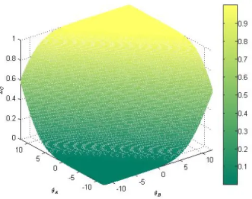
Figure 2 shows the share of agents picking option A. The number of agents choosing action A increases in θA and decreases inθB. IfθAincreases the distribution of signals on fundamental value A (xiA) shifts to the right. Thus the higher θA is, the more agents get signalxiA high enough (relative to the other signal,xiB) to pick action A. While when θB
decreases the distribution of signals on fundamental value B (xiB) shifts to the left, hence the cutoff for choosing option A decreases and thus more agents opt for action A.
Figure 2: Share of Agents Choosing Option A in the Separate-risky-option Case in the Space of Fundamental Values
4 Unified Options
4.1 Equilibrium
In the second scenario agents either choose the safe option or a risky option depending on the unified fundamentals, that is Ω ={0, C}. Again, I consider symmetric Bayesian Nash Equilibria with Bayesian pure strategy s:R2 →Ω, wheres(xi) is the action chosen if the agent receives the pair of signals xi = (xiA, xiB). In the equilibrium each agents pick the
the risky unified option if its expected payoff given her own pair of signals (xi) and others’
strategy (×j∈I/is(xj)) is higher than the payoff from the outside option.
An agent prefers the unified risky option to the safe option ifp(θC+LC)> o. Aspis strictly increasing, there exists a constantn≡p−1(o), such that the latter is equivalent to θC +LC > n.
Hence the strategy should be such that an agent opts for the unified option if and only if she expects θC +LC conditional on her own pair of signals (xi) and others’ strategy (×j∈I/is(xj)) to be higher than n. That is, for each xi ∈R2
s(xi) =
C ifE
θC+LC
xi,×j∈I/is(xj)
> n
0 otherwise
Let us definexiC ≡ 12 xiA+xiB
. Given the signal generating processes for xiA and xiB this can be rearranged toxiC = 12 θA+εiA+θB+εiB
=θC+εiC, withεiC = 12 εiA+εiB
= ei+12 eiA+eiB
. AsεiAandεiBare normal random variablesεiC is also distributed normally with mean 0 and standard deviationσC =
q
σ2+14σA2 +14σB2. One can show that the case of unified option is equivalent to the standard one dimensional case with fundamental value θC and private signal xiC = θC +εiC. This implies6 that there is always a unique equilibrium in switching strategies, such that agents choose the unified risky option if and only if xiC > n−12.
By using that xiC ≡ 12 xiA+xiB
, we can express the cutoff in terms of the original signals. Thus we get a cutoff functionkC0 xiA
=−xiA+ 2n−1, implying the strategy s(xi) =
C ifxiB> kC0(xiA) =−xiA+ 2n−1
0 otherwise (11)
4.2 Implications
The cutoff line characterized by Equation 11 is shown in Figure 3. It is in fact a straight line. Agents with a pair of signals falling on the area top right to this line opt for the unified option while others choose the safe option.
The aggregate number of agents choosing the risky joint option is given by the following equation:
E(LC|θ) =P(xiB > kC0(xiA)|θ) =
∞
Z
−∞
∞
Z
kC0(uA)
f(uA, uB)duBduA (12) where again, f(uA, uB) is the joint pdf ofxiA|θ and xiB|θ.
6For a proof see for instance Morris and Shin (2003).
Figure 3: Cutoffs for the Unified-risky-option Case in the Space of Private Signals Figure 4 shows the share of agents choosing the unified risky option. The share of agents picking the unified option is increasing in bothθA and θB. The higher any of the two fundamental values the more agent gets such signals that their sum is high enough to choose the unified risky option.
Figure 4: Share of Agents Choosing the Unified Risky Option in the Space of Fundamental Values
5 Comparison
In this section I compare different scenarios. In Subsection 5.1 I set the standard benchmark case when there is a single risky option with its own fundamental value against the case of two separate risky options. Then in Subsection 5.2 I compare the two-separate-risky- actions case with the unified-risky-options case, that is when there is one risky action depending on both fundamental values. In both subsections I first study the difference in the individual decision of agents, then I analyze the aggregate behavior of the agents.
5.1 One Single Risky Option Versus Two Separate Risky Options
Suppose there is a single risky option with its own fundamental value. In this case the cutoff is given by a constant, in our setupk=−0.5 +nis the cutoff value (see Morris and Shin (2003)). An agent chooses the safe option if her signal is smaller than the cutoff value and opt for the risky one if higher.
How does the decision of the agent change if instead of a single risky option there are two risky possibilities? Figure 5 compares the outcomes regarding action A as a function of the private signals.7 The lines on the graph are the cutoff functions. The areas determined by the lines are denoted by two letters of which the first indicates the choice in the single- risky-action case, while the second indicates the outcome when there are two risky options.
Figure 5: Comparison of the Individual Decisions in the Single-risky-option and Two- separate-risky-option Cases
7Note thatxiB does not influence the decision of the agents when they can only choose action A, still I present the result in thexiA-xiB space to be comparable with the two-risky-action case.
The vertical line atn−0.5 is the cutoff in the single-risky-option case. With a private signal smaller thann−0.5 (the area left to this line) the agents do not pick the single risky option. Note that this decision is not influenced by the availability of another risky option.
Indeed, with such signals she picks risky action A neither in the single-risky-option, nor in the two-separate-risky-option case. The only difference is that when there is a second risky possibility that the agent expects to be attractive enough (her private signal on action B is higher thankB0) she pick that option (see the area denoted by 0-B), which she cannot in the single-risky-option case. Otherwise she keeps choosing the outside option (area 0-0).
When the agent receives a signal above n−0.5 (area right to the line) she picks the single risky option. This action may change when there is another risky possibility. First, she may prefer to take the other risky alternative. With private signals falling on the domain A-B the agent has an expected gain from choosing option B higher than both the outside option and the gain from picking option A. Second, she may also prefer to choose the outside option. Area A-0 shows the pair of signals with which an agent does not choose neither of the two risky options though opt for the single risky option. This domain is enclosed by kB0, kA0 and −0.5 +n lines. Proposition 5 states that this area indeed exists (see the proof in the Appendix).
Proposition 5 (inert area). The cutoff functions are above the −1/2 +n line, that is kr0(xi−r)>−0.5 +n for r∈ {A, B} and xi−r∈R.
This area reveals that when there is a second option, however, not attractable for an agent, she is less willing to choose the first option. This is because agents have incentives to make mutually consistent actions. Given that the number of agents is fixed, when there are multiple options, their power is split. The more agent coordinates on one option the less people there are who can potentially coordinate on the other. This generates a negative correlation between the two options. I refer to this endogenous correlation as strategic correlation. Given that the fundamentals are uncorrelated, without the strategic correlation the willingness of an agent to pick a risky option should not be influenced by her expectations about the fundamental value of the other risky option that she will not choose for sure. Still, due to the endogenous strategic correlation, the availability of a second option, even when not attractable for an agent, makes the agent less willing to choose the first option.
Let us turn to the aggregates and compare the overall number of agents choosing option A under the two scenarios. Equation (10) and Figure 2 show the share of agents choosing option A in the two-separate-risky-option case. In the single-risky-option case the share of agents picking the risky option can be simply calculated by using the properties of a one dimensional normal distribution (see Morris and Shin (2003)). For a givenθAfundamental value the share of agents taking action A is given by the following equation
E(LA|θA) =P(xiA>−1/2 +n) = 1 σA
Φ
θA+ 0.5−n σA
(13)
where again Φ (z) denotes the cdf of the univariate standard normal distribution.
Figure 6 compares the share of agents who choose action A if there are two separate risky and a safe option versus if besides the safe option only risky action A is available (LA−L). The outcomes are plotted in the space of fundamentals8. The left panel shows the 3-dimensional surface while the right panel shows its contour projection on the XY plane.
Figure 6: Comparison of the Aggregate Number of Agents Choosing the Single Risky Option and Either of the Two Separate Risky Options
When θA is low enough the agents would not pick action A in neither case, thus the presence of the second risky option does not influence the outcome. However, when θA is higher the availability of risky option B matters. In particular the higherθB is relative to θA, the less agents pick option A as they rather choose option B.
5.2 Two Separated Versus Two Unified Risky Options
In this subsection I compare the cases when the two risky options are separated and when they are unified. Figure 7 shows the individual decisions as a function of private signals in both cases. The lines on the graph are the cutoff functions. Similarly as before, thekA0, kAB and kB0 lines show the cutoff lines in the two-separate-risky-option case. While kC0 shows the cutoff line for the unified-risky-option case.
The areas determined by the lines are denoted by two letters of which the first indicates the choice when there are two separated risky possibilities, while the second indicates the outcome when they are unified. Agents with pair of signals falling on the 0-0 domain choose the outside option in both cases. Then, agents in domains A-C and B-C pick one of the separate risky options (at A-C they opt for action A, while at B-C they choose option B) and also the unified risky option. At the same time, agents with pair of signals on area A-0 or B-0 choose the risky option A or B, respectively, but does not choose their union.
8Note thatθB does not influence the outcome in the single-risky-option case, still I present the result in theθA-θB space to be comparable with the two-risky-option case.
Figure 7: Comparison of Individual Decisions in the Separate-risky-option and the Unified- risky-option Cases
These areas include agents who receive high signal about one of the fundamentals and low about the other. Hence, these agents expect one of the options to be valuable enough for choosing of its own, however the low expected value of the other option makes unattractive the unified option. Finally, agents with private signals on the area 0-C choose neither of the separate risky options but pick their union. This is due to the fact that the negative strategic correlation is present in case of separate options but not in case of unification.
Indeed, when there are two separate risky possibilities there are two potential targets to coordinate on, hence the coordination disperses and thus weakens its power. While in case of a unified risky option agents coordinate on a single target, thus the negative strategic correlation does not arise. It is easy to show that the 0-C area indeed exists by using Proposition 5 and the observation that the linekC0 crosses the (n−0.5, n−0.5) point.
Let us turn to the aggregate behavior of the agents. Equation (10) and Figure 2 show LA, the share of agents choosing option A in the case of two separate risky options. While if the risky options are unified the aggregate number of agents choosing it is shared, that is LA=LB = L2C, where Equation (12) and Figure 4 showLC, the share of agents choosing the unified option.
Consider first the overall number of agents choosing any of the risky possibilities. Fig- ure 8 shows the difference between the total number of agents choosing a risky option in case of joint and separate risky options (LC −LA−LB). The outcomes are shown in the space of the fundamental values of the two options. The top left panel shows the 3-dimensional surface while the top right panel shows its contour projection on the XY plane while the bottom panel shows the sign of the difference.
Figure 8: Comparison of the Aggregate Number of Agents Choosing the Unified Risky Option and Either of the Risky Options
The sign is positive when more agents pick the unified option than the two separate risky options and negative in the reverse case. The difference is around zero when the unification does not influence the total number of agents choosing them. There are two such typical situations: first, when one of the fundamentals is so high that it outweighs the other fundamental value (see the northeast part on the top right panel); second, when both fundamentals are low (see the southwest part on the top right panel). In the former case, the option with high fundamental value dominates the union, which is thus chosen with similar intensity, while the other option alone is not selected. In the latter case, none of the separate risky options and neither their union is picked. More agents choose either of the independent risky options than their union (see the dark areas on the top right panel) when one of the risky option has high fundamental value and the other has low, but in absolute value the one with low is greater. In this case the option with high fundamental value is chosen, but not the union. However, there are situations when slightly more agents opt for the joint option than in either of the separate risky options (see the light area on the bottom panel). This is the case when the value of the two fundamentals are close to each other and both are low. In this situation, because of the negative strategic correlation, a
single target is more attractive than multiple targets, this is why more agents choose the union of the risky options than the distinct options.
Consider next how the form of the risky options affects, say, option A. Figure 9 shows the difference between the number of agents assigned to option A in the unified and in the separated case (LC/2−LA). The outcomes are shown in the space of fundamentals.
The left panel shows the 3-dimensional surface while the right panel shows its contour projection on the XY plane.
Figure 9: Comparison of the Aggregate Number of Agents Assigned to Option A in the Separate-risky-option and the Unified-risky-option Cases
The figure reveals that when bothθAandθBare low (see the southwest part on the right panel) the form of the risky options does not make a difference, since neither fundamental A individually, nor the alliance of the two fundamentals is chosen. However, when θA is high compared toθB (see the north and the northwest part on the right panel) less agent picks the union as fundamental B counteracts the strength of fundamental A, so in these cases option A is less popular individually. Meanwhile, when θB is high compared to θA
(see the east and the southeast part on the right panel) more agents pick option A singly as the lower fundamental value of B makes the union less preferred.
6 Information Accuracy
This section shows how the outcomes depend on the information precision. I investigate what happens if the standard deviation, either the systematic part (s) or the fundamental specific parts (sAandsB), of the noise term changes. Higher standard deviation means that there is lower information in the signals. The information precision affects the individual decisions when there are separate risky options, but does not affect when they are unified.
However, the aggregate behavior of the agents changes in both scenarios.
First, I consider changes in the standard deviation of the systemic part of the noise term (s). Figure 10 provides a geometrical representation of how the cutoff lines separating the
Figure 10: Cutoff Lines in the Two-separate-risky-option Case at Various Standard Devi- ations of the Systemic Part of the Noise Term (s={1,2,4} andsA=sB= 0.7)
potential choices of an agent shifts for differentsvalues. The fundamental specific variances are fixed at sA=sB= 0.7.
The plot reveals that when s increases, the cutoff lines kAO and kBO shift equally outwards from the -0.5 lines. So the higher the uncertainty, the higher signal on a given option is needed for an agent to choose that option. The intuition is the following: the higher dispersion of the expectation of the fundamentals makes the agents to expect that a larger share of their fellow agents would pick the other risky option. In other worlds, higher uncertainty makes coordination harder, thus strengthens the negative strategic correlation, and therefor enlarges the inert area.
Figure 11 shows how the value ofsinfluences the aggregate number of agents choosing option A in the separate-risky-option case (LA, see Subfigure 11a) and in the unified-risky- option case (LC, see Subfigure 11b).
Assincreases both curves become flatter, so the higher uncertainty reduces the potency of the fundamentals. This is also reflected in the difference between the aggregate behavior of the agents under the two scenarios, which is also plotted on Figure 11. Subfigure 11c plots the difference between the number of agents choosing option A in case of unified and separate risky options (LC/2−LA). Subfigure 11d shows the difference between the total number of agents who opt for the unified risky option and who pick either of the separate risky options (LC−LA−LB).
Both flatten and drift towards zero as s increases. In other worlds, when the agents’
private information is more accurate, the difference between the agents’ aggregate behavior under the various scenarios decreases.
Note that all the effects caused by changes insare symmetric in the two risky options.
(a)LA (b)LC (c)LC/2−LA (d)LC−LA−LB
Figure 11: Aggregate Number of Agents and Differences Between the Aggregate Number of Agents Choosing the Different Options at Various Standard Deviations of the Systemic Part of the Noise Term (s={1,2,4} and sA=sB= 0.7)
Now, I bring in asymmetry and consider variation in the standard deviation of the option specific part of the noise. Figure 12 shows how the cutoff lines in the separate-risky-option case vary depending on the value of sB. The other parameters are fixed at sA = 0.7 and s= 2.
When information on option B is less accurate (that is sB increases), the three cutoff lines move to higherθB and lower θA values. This is in line with the previous finding that the cutoff lines shifts upward when there is higher uncertainty. Indeed,kBO shifts upward as higher sB means bigger uncertainty regarding option B. Meanwhile, an increase in sB
decreases the relative (compared to option B) uncertainty about option A, that is whykAO shifts downward.
Figure 13 plots the agents aggregate behavior for various sB values. Subfigure 13a shows the aggregate number of agents picking option A in the instance of separate risky options (LA), while Subfigure 13b shows the share of agents choosing the unified risky option (LC).
Changes insB twist theLAsurface, but notLC. This is because due to the unification all effects are divided equally, thus even the option specific changes have symmetric effects and affect only the steepness but not the curvature ofLC.
But, given thatLArotates, the difference of the share of agents assigned to a risky option under the different scenarios rotates as well. This is shown on Figure 13. Subfigure 13c
Figure 12: Cutoff Lines in the Two-separate-risky-option Case at Various Standard Devia- tions of the Option Specific Part of the Noise Term (s= 2,sA= 0.7 andsB ={0.6,0.7,3})
(a)LA (b)LC (c)LC/2−LA (d)LC−LA−LB Figure 13: Aggregate Number of Agents and Differences Between the Aggregate Number of Agents Choosing the Different Options at Various Standard Deviations of the Option Specific Part of the Noise Term (s= 2, sA= 0.7 and sB ={0.6,0.7,3})
plots the difference between the agents assigned to option A in case of joint and separate options (LC
2 −LA). Subfigure 13d compares the total number of agents who choose the joint risky option and who pick either of the separate risky options (LC−LA−LB).
7 Applications
In this section I show two potential applications of the multidimensional global games model. First, in Subsection 7.1 I describe a model for the choice of oil invoicing currency.
Second, in Subsection 7.2 I present a model for the issuance of the European common bond.
7.1 Choice of Currency for Oil Invoicing
In this subsection I introduce a model that describes the choice of invoicing currency in the oil market. The model is an extended, but partially simplified version of the model developed by Mileva and Siegfried (2007).9 There is a continuum of crude oil seller with measure one, indexed byi∈I = [0,1]. Oil sellers have to decide which currency to use for invoicing their oil contracts. Suppose there are three currencies, the US Dollar, the Euro and the British Pound, which can be used, that is j ∈ {U DS, EU R, GBP}. Each seller can use only a single currency. In time t= 1 sellers decide on the currency, while at time t= 2 trade takes place and sellers realize their income. The price of oil is independent of the invoicing currency, however the cost varies depending on the currency.
The cost of using currency j is Cj. It contains the transaction cost, the liquidity cost and the information cost. Information cost arises only for the Euro and for the British Pound. In the oil market the historically established invoicing currency is the US Dollar.
However, switching to a different currency have information cost as the traders have to learn the usage of the new unit of account. The more trader uses the new currency the lower the information cost is. I assume that the transaction and the liquidity cost do not depend on the number of traders using the given currency,10 hence the cost of usage is the function of the number of agents who use the currency for the Euro and for the British Pound but not for the US Dollar. The aggregate number of agents using currency j is denoted byLj, while cj is the part of the cost of using currency j which does not depend on the aggregate number of users. For simplicity, I assume thatLj enters the cost function in an additive way. Thus the cost functions areCU SD=cU SD,CEU R =cEU R−LEU R and CGBP =cGBP −LGBP.
9Their emphasis is on the network effects which arise from the assumption that currency choice of crude oil sellers determine the currency distribution of other goods. I exclude this assumption and rather build on the learning element of the model.
10Contrary to the model in Mileva and Siegfried (2007) I suppose that the denomination of oil producers’
expenses is not influenced by the composition of the invoicing currency of oil as the oil market is small compared to the non-oil market.
At t = 1 sellers get noisy signals Xji = cj +ij for each j ∈ {U SD, EU R, GBP}, whereij are the noise terms which are distributed independently and normally with mean 0 and standard deviation ςj, and are independent across agents. Given her signal triplet each seller decides on her invoicing currency choice. A seller prefers the Euro over the other two currencies if she expectscEU R−cU SD−LEU R to be negative and smaller than cGBP−cU SD−LGBP. Similarly, a seller prefers the most the British Pound if she expects cGBP −cU SD−LGBP to be negative and smaller than cEU R−cU SD−LEU R. Otherwise, she prefers the most the US Dollar.
Let me introduce the notationsθr≡cU SD−crandxir≡XU SDi −Xri,εir =iU SD−ir for r∈ {EU R, GBP}. Such we have the same model as described in Section 2. In particular the two risky options are the Euro and the British Pound and the US Dollar is the outside option. The two fundamental values are θEU R and θGBP on which oil sellers get signals xiEU RandxiEU R, whereiU SDis the systematic part and−iris the fundamental specific part of the noise terms. Thus the standard deviations areσEU R =
q
ςU SD2 +ςEU R2 andσGBP = q
ςU SD2 +ςGBP2 , while the correlation coefficient is ρ = ς
2 U SD
q(ςU SD2 +ςEU R2 )q(ςU SD2 +ςGBP2 ). Fi- nally, one can get from the payments after some algebra thatn= 0.
Let me compare the individual decisions when only the Euro and when both the Euro and the British Pound are available besides the US Dollar for invoicing oil contracts.
Figure 5 is suitable for the comparison. Option 0 represents the US Dollar, option A is the Euro and option C is the British Pound. The line at−0.5 (since n= 0, n−0.5 =−0.5) separate the traders decision when only the US Dollar and the Euro are usable. In the three-currency-case the kB0, kBA and kA0 lines separate the traders’ decisions. A trader withxir≡<−0.5 (left to the line at−0.5), or equivalentlyXU SDi < Xri−0.5, switches to the Euro, otherwise continues to use the US Dollar in the two-currencies case. How does the availability of another currency (in our example the British Pound) affects the traders’
decision on the invoicing currency? Oil sellers using the US Dollar in the two-currencies case either continue to use the US Dollar (0-0 area) or switches to the British Pound (0-B area). Traders who switch to the usage of the Euro when this is the only new currency besides the US Dollar either choose again the Euro (A-A area) or switch to the British Pound (A-B area) or after all use the US Dollar (A-0 area). Hence there are situations when an oil seller would switch to the usage of a new currency if there were one new currency besides the US Dollar, however would not switch if there were two other currencies.
7.2 Introduction of the Common European Bond
In this subsection I present a model to describe the introduction of a joint bond that would replace the national issuance by member states of the Eurozone. Here I concentrate on the case when symmetric countries issue the common bond. For this, the model with uncor- related fundamentals is suitable. To assess the case of asymmetric countries a model with