Technical review on derivation methods for behavior dependent functional responses

(1)

Community ECology 20(1): 28-44, 2019 1585-8553 © The Author(s).

This article is published with Open Access at www.akademiai.com DOI: 10.1556/168.2019.20.1.4

1. Introduction

Time constraint appears almost everywhere in biology, e.g., in different stages of ontogeny (such as offspring care, insect metamorphosis), territorial defense, fighting and sleep- ing, etc. In the review, I concentrate on the time constraint of feeding. The main point is that handling time can decrease the predation press on the prey population, since handling time decreases the number of active predators in the population. The aim of this technical review is to survey the different mathematical methods of the derivation of functional responses, mainly focusing on the effect of time constraints and the behavior of prey and predator. Consequently, this review does not intend to collect all functional responses that have been proposed (cf. Jeschke et al. 2002). Furthermore the question is not considered whether an already proposed functional response is viewed as reasonable from a biological viewpoint (see e.g., Fenlon and Faddy 2006, Jost and Ellner 2000). For instance, how to incorporate exactly the effect of predator density on the functional response remains somewhat controversial (e.g., Abrams 2014, Arditi et al.

1991, Arditi and Ginzburg 2012, Hossie and Murray 2016, Kalinoski and DeLong 2016, Kratina et al. 2009). Moreover,

this review does not discuss the problem of conditions under which existing functional response can be applied to concrete biological cases (e.g., Tellez et al. 2009).

In the introduction, the following questions are considered: firstly, why is functional response one of the major is- sues in ecology? Secondly, why is the behavior of predator and prey crucial in the functional response, and what is the relationship between the functional response and optimization theory and/or game theory? Finally, a simple description of predation process is also given, which is the starting point of most derivation methods of functional responses.

1.1. Why is behavior-dependent functional response important?

Functional response (Solomon 1949) is the average number of food prey eaten by an arbitrary predator individual per unit time. In the broadest sense, the term “predator” means

“forager”, i.e., carnivore, omnivore, herbivore, parasites or parasitoids. In this paper, I will use the term predators in this sense. Similarly, in this general sense, prey will mean the food of the considered predator. Clearly, the functional response measures the negative effect of the predator species

Technical review on derivation methods for behavior dependent functional responses

J. Garay

MTA Centre for Ecological Research, Evolutionary Systems Research Group, Klebelsberg Kunó u. 3, H-8237 Tihany, Hungary

and MTA-ELTE Research Group in Theoretical Biology and Evolutionary Ecology and Department of Plant Systematics, Ecology and Theoretical Biology, ELTE Eötvös Loránd University, Pázmány Péter sétány1/c, H-1117 Budapest, Hungary. Phone: +36 1 3722500/8798, Fax: +36 1 3812188. E-mail: garayj@caesar.elte.hu

Keywords: Markov chain, Renewal process, Stage dynamics, Time constraint, Wald’s equality.

Abstract: Functional responses measure the trophic interactions between species, taking into account the density and behavior of the interacting species. In predator-prey interactions, the prey preference of the predator and the antipredator behavior of the prey together determine the feeding rate of the predator and the survival rate of the prey. Consequently, the behavior dependent functional responses make it possible to establish dynamic ecological models providing insight, among others, into the coexist- ence of predator and prey species and the efficiency of agents in biological pest control. In this paper the derivation methods of functional responses are reviewed. Basically, there are three classes of such methods: heuristic, stochastic and deterministic ones. All of them can take account of the behavior of the predator and prey. There are three main stochastic methods for the derivation of functional responses: renewal theory, Markov chain and the Wald equality-based method. All these methods assume that during the foraging process the prey densities do not change, which provides a mathematical basis for heuristic derivation.

There are two deterministic methods using differential equations. The first one also assumes that during the foraging process the prey densities do not change, while the second one does not use that assumption. These derivation methods are appropriate to handle the behavior dependent functional responses, which is essential in the derivation of ecological games, when the payoff of prey and predator depends on the strategies of the prey and predator at the same time.

(2)

Derivation of functional responses 29 on the prey species. The numerical response (Solomon 1949)

is the number of offspring (e.g., newborn, eggs or biomass growth rate) of a single predator per unit time. The numerical response depends on the prey eaten by a single predator. Thus it is a function of the functional response (cf. Garay et al.

2012, 2018). Consequently, functional response is the most essential component in trophic interactions, since it describes the intensity of the trophic connections.

Functional response is an important component in the following basic questions of theoretical ecology: when do trophically linked species coexist? Since all food webs are formed by trophically linked species, the question arises: when is a food web stable (Uchida et al. 2007, Valdovinos et al. 2010)?

Now this question also arises: why are the behaviors of the prey and the predator important in this issue? In theoretical ecology, one of the possible mechanisms for maintaining di- versity is negative frequency-dependent selection, i.e., rare prey experience higher survival than more common types (see e.g., Merilaita 2006, Punzalan et al. 2005). Clearly, in the predation process, predators’ prey preference (cf. switching in the optimal foraging theory, Stephens and Krebs 1986, Krivan and Sikder 1999, and see Murdoch et al. 1975, van Baalen et al. 2001) implies negative frequency-dependent selection. Thus, the question arises: can the adaptive behavior of prey or predator stabilize the trophic interaction (Kondoh 2003, 2006, Valdovinos et al. 2010)? For an answer to the latter question, first we have to understand the effect of the adaptive behavior of prey or predator on functional response.

For instance: What kind of prey preference maximizes the numerical response of a predator (see optimal foraging theory, Stephens and Krebs 1986)? Moreover, can the antipredator behavior of prey stabilize the food web (Kondoh 2007)?

When is density dependent mutualism stable (Holland et al.

2002, Holland and DeAngelis 2010)? The above listed questions call the attention to the importance of the behavior dependent functional responses.

Moreover, the functional response is an important issue also from the view point of biological pest control. Does a given agent (predator, parasite species) effectively control the density of a given pest? (See e.g., Cabello et al. 2007, Lester and Harmsen 2002.) In biological pest control, the tempera- ture dependence of the functional response is also important (Garcia-Martín et al. 2008), and the functional response of a given predator also depends on the prey types (Tellez et al.

2009).

In summary, the functional response is important in both theoretical and applied ecology.

1.2. Aspects of a possible classification of functional responses

Holling has already classified the functional responses according to the different linear and non-linear dependence on the density of a single prey species. The corresponding Holling types I-IV functional responses are well known (see Section 3.3).

This classification is based on the shape of the functional response. However, the predation process is not a simple one, thus the classification of the existing functional responses is not an easy task. For instance, Jeschke et al. (2002) classify and give the family tree of different 34 functional responses.

Although the classification of all functional responses is not the aim of the present paper, I call attention to two aspects of functional responses. The main point is that functional response depends on the density and the behavior of prey and predator, simultaneously. Thus, from the point of view of the present paper, there are at least two basic aspects of a possible classification of functional responses:

Aspect 1. The density of how many species has effect on the given functional response (see e.g., Abrams and Ginzburg (2000): 1. The functional response is single prey dependent, when prey density alone determines the response (e.g., Holling I, II and III functional response, see Section 3.3). 2.

The functional response is prey-predator dependent, when both predator and prey populations density affect the response (e.g., Beddington –DeAngelis functional response). 3.

The functional response is multispecies dependent, when species other than the focal predator and its prey species influ- ence the functional response. In this paper we do not consider this case when a third species, namely parasite, modifies the functional response (Toscano 2014).

Aspect 2. Do the behaviors of interacting species have an effect on the given functional responses? The importance of Aspect 2 is that the theoretical models taking account of the behaviors of predators and prey have to use quite different mathematical tools to find the optimal behavior of predator and/or prey. Here there are four main possibilities.

2.1 No behavior effect. The behaviors of interacting species have no effect on functional response (see e.g., Holling II type in Section 2.1). This is the simplest case, there is no optimization problem and the functional response depends only on the density of prey.

2.2 Only predator’s behavior has effect on its functional re- sponse without interference between predators. If there is no interaction between predators during the foraging process, and each predator has two different prey species, then the prey preference of the predator determines the functional responses (Stephens and Krebs 1986). The most studied problem in this case is how the predator’s preference maximizes its numerical response. Optimal-foraging theory postulates that the forager maximizes its average net energy intake per unit time (Andersson 1981, Charnov 1976, Stephens and Krebs 1986, Turelli et al. 1982). The well-known zero-one rule of optimal foraging theory (either always attack or always ignore a prey type in the diet according to the actual density of different prey types) is one of the best examples for the way that predator behavior affects the functional response (Charnov 1976).

A consequence of the zero-one rule is the negative frequency- dependent selection, since the more abundant but less valuable prey type is attacked by the predator, if the density of the more valuable prey is low, so the predation pressure on the rare but more valuable prey type decreases.

(3)

30 Garay 2.3. Only the prey’s behavior has an effect on the predator's

functional response. Clearly, the prey behavior can have an effect on the predator’s success. Such kind of antipredator behavior is refuge using (Cressman and Garay 2009, Hossie and Murray 2010, McNair 1987, Sih 1987), crypsis (Erichsen et al. 1980), mimicry (Real 1977), herd formation (Cosner et al.

1999, Eshel 1978, Cressman and Garay 2011), habitat preference (Cressman et al. 2004) and active defense (e.g., Hammill et al. 2010). For instance, elephants and buffalos can actively defend themselves and their young against lions, and they can kill lions (Hayward and Kerley 2005).

It is important to point out here that there is an essential difference between the mathematical tools needed when the functional response exclusively depends on either prey or predator behavior.

When the predator’s payoff does not depend on another predator’s strategy and the preys’ antipredator strategies, then the predator optimizes its foraging strategy (see classical optimal foraging theory, e.g., Stephens and Krebs 1986). When the prey use different antipredator strategies and the fixed predator’s prey preference determines the survival rate of different antipredator strategy, then the survival rate of each prey type depends on the antipredator strategies used by the whole prey population (independently of whether predator can change its foraging strategy). In other words, the survival rate of a given prey type depends on the strategies used by other prey (Garay et al. 2015b); in which case a population game (Broom and Rychtar 2013, Brown and Vincent 1992) has to be used for the prey population (Garay et al. 2015b).

I note that this selection situation for the prey is similar to apparent competition (Holt and Bonsall 2017) when the individuals from different prey species have no direct competition, but the common predator indirectly connects these species, since in one prey species the survival rate increases when the predator mainly consumes the other prey species.

For an example of this kind of game, see Saleem et al. (2006) where, for a two predator one prey system, an evolutionar- ily stable strategy for the prey’s defensive switching is given.

Moreover, when Broom and Krivan (2018) surveyed the habitat selection game, they concentrated on functional responses of Holling types I and II.

2.4 Only predator’s behavior has an effect on its function- al response with interference between predators. If there is interaction between predators during the foraging process, then there are two cases. For the first case the Beddington- DeAngelis functional response is a good example, where the interaction is not connected directly to the feeding, but the time constraint of the interaction decreases the total time duration of foraging, consequently the interaction time decreases the number of killed prey (see Section 3.3). For instance, the fight between predators clearly decreases the functional response (Garay at al. 2015a). In the second case, the interactions are connected to feeding. For instance, Auger et al.

(2002) started from the classical hawk and dove game, when predator individuals can use two behavioral tactics to dispute a prey when they meet, and used Holling type I functional response. In kleptoparasitism (Iyengar 2008), fighting for the killed prey takes time, thus kleptoparasitism also decreases

the predation pressure on prey. In summary, in the first case the optimization models are used to find the optimal behavior of the predator, while in the second case a game theoretical model is needed (Broom and Rychtar 2013).

2.5. The preys’ and predators’ behavior together have effect on the functional response. Clearly, Aspects 1 and 2 take place at the same time. For instance, the evolution of mimicry is a multi-species problem, where the predator’s prey preference and the phenotypic similarity between two prey species together determine the evolutionary success of the different phenotypes of different prey species and the predator, as well (e.g., Getty 1985, Sherratt 2002). Furthermore, in Serengeti a pride of lions are hunting on gregarious prey and this group formation has an effect on the functional response (Fryxell et al. 2007, Krivan et al. 2008). If the preys’ antipredator strategy and predators’ prey preference have effect on the functional responses simultaneously, then a multi species, density dependent population game can be given by the behavior and density dependent functional response (Cressman et al. 2004, Garay et al. 2015b), since the prey and predator behavior together determine the functional response. Now I mention some game theoretical models for predator-prey interactions.

Group formation has an effect on the survival of prey and energy gain of predator (Cressman and Garay 2011, Lett et al. 2004). Habitat usage also determines the predator’s success (Cressman et al. 2004, Hammond et al. 2007, Holt 1985, Hugie and Dill 1994). Prey refuge usage increases the survival rate of prey (Molla et al. 2018, van Baalen and Sabelis 1993). Game theory is not only important in the predation process (e.g., Abrams et al. 1993, Brown et al. 1999, Vardi et al. 2017). For instance, in the plant-pollinator connection, the species are also counter-interested (e.g., Wang et al. 2012, Garay et al. 2003).

1.3. Time constraint and predation cycle

For the sake of simplicity (e.g., for the simplest figures and equations), here we consider only 3 main stages of the predation cycle, but these stages can be subdivided into fur- ther stages.

1.3.1. Search (traveling, encounter and recognition), when the predator is looking for its prey. This stage begins when the predator starts to look for food and ends when the predator finds its prey. Clearly, this stage includes the traveling, the local searching in a perception range and the recognition of prey type.

The traveling by predator is determined by the habitat preference of prey (Garay et al. 2018). There are two main factors determining the ideal free distribution of prey: firstly, the habitats give different food supply (Fretwell and Lucas 1970). Secondly, in different habitats the predation pressure is different according to the different properties of the habitat (Krivan and Schmitz 2003).

The local searching in a perception range also depends on the phenotype of the prey and the behavior of the predators.

For instance, when the prey is cryptic, the predator can use its search image (Garay et al. 2018, Tinbergen 1960).

(4)

Derivation of functional responses 31 The recognition of a prey type also depends on the pheno-

type of the predator and its prey (Kotler and Mitchell 1995).

For instance, during the evolution of mimicry, the recognition of the palatable prey is an important factor (MacDougall and Dawkins 1998).

1.3.2. Attacks and killing. This stage starts when the predator attacks prey and ends when the predator has either killed or missed its prey. At this stage, the behaviors of the predator and its prey, together determine the success of the predator.

Firstly, after the recognition of encountered prey, predator, according to its own prey preference, does or does not attack the prey. Secondly, the prey antipredator behavior has an effect on the success of the attack by the predator. For instance, refuge usage and gregarious behavior of the prey can also decrease the predator’s success, and in some cases the active defense against predator is also successful.

1.3.3. Handling. This stage starts with either chop up, trans- port or eat and digest the food. During this stage the interaction between predators, e.g., kleptoparasitism (Wittenberger and Hunt 1985) or scrounge game (Barta and Giraldeau 2000) may happen.

Observe that a predation turn of the predator may end with several events: when the handling stage ends, when the predator has found not preferred prey, when the predator has missed the prey so the attacked prey survives, etc. The common feature of these three stages is time constraint, namely each predator spends time in these stages. After the predator has finished its turn, it starts a new turn, and so on, during the predation time duration T.

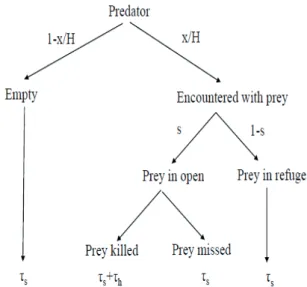
Based on the assumption that the different predator stages are mutually exclusive, the predation process form a predation cycle with different predation turns (see Fig. 1).

The structure of this paper is the following: Firstly, the heuristic derivation method is presented. Secondly, the stochastic methods are overviewed. Thirdly, the deterministic mathematical tools are surveyed. In each section a few applications are delineated, but a total overview is impossible, since there are too many of them. Finally, a short discussion is presented.

2. Heuristic time-budgeting argument

Since Holling used a heuristic argument when he introduced his functional response, I start with this derivation method. First, the original derivation of Holling is presented, then a more general heuristic reasoning is given.

2.1. Holling’s discs equation

First we briefly recall the original derivation of Holling type II functional response by Holling (1959a,b). Consider a predator foraging during time duration T. The predator is either searching for a prey or handling a prey. Holling used the following assumptions:

A) The searching and handling exclude each other, and both need time: Let τ_h denote the average handling time of one prey individual. Then during T we have two time dura- tions: T_s and T_h the total time duration of searching and handling, respectively, so T_s + T_h =T.

B) Assume that during T the finding rate of a prey does not change, let us denote it by a. We note that this assumption is valid if during T the density of prey (denoted by x) is not changed by the predator.

C) There is a linear relationship between finding a prey and the prey density, i.e., if the prey density is doubled, the killing probability is also doubled. Formally, px is the killing rate if the prey density equals x during T. We note that px is the average number of killings per time unit, and this is the reason why Holling’s original derivation does not include the searching time.

Denoting the consumed prey by y, based on Assumption C, we have

1 2

pxTS

y . (1)

3

is pxTs. Moreover, since the handling time of a single prey, h determines the 4

searching time, we also have 5

y T

T_S _h . (2)

6

Substituting (2) into (1) we get 7

)

(T y

px

y h , (3)

8

which simplifies to 9

px h

y pxT

1 . (4)

10

Thus, with T=1, we have 11

px h

y px

1 . (5)

12 13

14 15

T

T F_itheaveragenumber ofkilledi-th prey during . 16

(1) Indeed, since px is the average killing per unit time, during T_s the number of killed prey is pxT_s. Moreover, since the handling time of a single prey, th determines the searching time, we also have

1 1

2

pxTS

y . (1)

3

is pxTs. Moreover, since the handling time of a single prey, h determines the 4

y T

T_S _h . (2)

6

)

(T y

px

y h , (3)

8

px h

y pxT



 

1 . (4)

10

px h

y px

1 . (5)

12 13

14 15

T

(2) Substituting (2) into (1) we get

1 1

2

pxTS

y . (1)

3

y T

TS h . (2)

6

)

(T y

px

y h , (3)

8

px h

y pxT

1 . (4)

10

px h

y px

1 . (5)

12 13

14 15

T

(3) which simplifies to

1 1

2

pxTS

y . (1)

3

is pxTs. Moreover, since the handling time of a single prey, h determines the 4

y T

T_S _h . (2)

6

)

(T y

px

y h , (3)

8

px h

y pxT

1 . (4)

10

px h

y px

1 . (5)

12 13

14 15

T

(4) Thus, with T=1, we have

1 1

2

pxTS

y . (1)

3

y T

T_S _h . (2)

6

)

(T y

px

y h , (3)

8

px h

y pxT

1 . (4)

10

px h

y px

1 . (5)

12 13

14 15

T

(5) Although Holling (1959a) originally considered an artificial

“predator-prey system”: a human “predator” is searching for paper discs on the table, for the perspective of model build- ing, in terms of the usual predation, Holling’s model has the following important assumptions:

1. The predator’s stages exclude each other, e.g., at a par- ticular time each predator is either searching or handling but cannot do these two activities simultaneously.

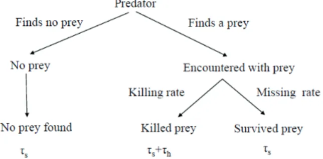
Figure 1. One turn of predation cycle, from starting a search to starting a next search, can be described by this tree. The searching and handling stages of the predator take time τs and τh, respectively. More details of predation process are given in Lima and Dill (1990).

11 1

2

Figure 1. One turn of predation cycle, from starting a search to starting a next search, 3

can be described by this tree. The searching and handling stages of the predator take 4

time τs and τh, respectively. More details of predation process has been found in Lima 5

and Dill (1990).

6 7 8

The structure of this paper is the following: Firstly, the heuristic derivation method is 9

presented. Secondly, the stochastic methods are overviewed. Thirdly, the deterministic 10

mathematical tools are surveyed. In each section a few applications are delineated, but a 11

total overview is impossible, since there are too many. Finally, a short discussion is 12

presented.

13 14

2. Heuristic time-budgeting argument 15

Since Holling used a heuristic argument when he introduced his functional response, I 16

start with this derivation method. First, the original derivation of Holling is presented, 17

then a more general heuristic reasoning is given.

18

(5)

32 Garay 2. There is a time constraint, i.e., each disjoint action of

predator needs time.

3. The killing rate depends on the density of prey.

4. During the investigated time period T, the density of prey does not change.

Although Holling’s model is the simplest description of the problem, these motives of Holling’s model are the basis of all mathematical derivation tools of functional response, reviewed below.

2.2 Heuristic argument for fixed prey density

There are three different time scales in the problem of predation. The first one is the longest one, the population growth time scale, which measures the densities change of predator and prey populations. This population dynamical time scale is significantly longer than that over which the functional response is measured (Abrams and Ginzburg 2000, Krivan and Cressman 2009). The second time scale, a smaller one is the time duration of predation cycles T. During T the density change by predator can be neglected. The third time scale, the shortest one is the time unit for measuring the different time duration of different stages of the predation cycles. In most derivation methods of functional response, the population dynamics time scale does not take place.

Basic assumption: The following heuristic argument is strict- ly based on the widely used assumption that during T, the predator's behavior and the preys’ density and the preys’ behavior do not change (see later in Section 3). The definition of functional response (i.e., the average number of food prey eaten by an arbitrary predator individual per unit time), reads as

1 1

2

pxTS

y . (1)

3

y T

T_S _h . (2)

6

)

(T y

px

y h , (3)

8

px h

y pxT



 

1 . (4)

10

px h

y px



 

1 . (5)

12 13

14 15

T

What is the average number of killed i-th prey during T? For an answer to this question, let us consider what an observer can see? During T, each focal predator has a random sequence of predation turns and kills i-th prey in only part of these predation turns. Thus, the first question arises: what is the average number G of different predation turns of a focal predator during T? For an answer to this question, let us calculate the average time duration of a predation turn (denote it by E(τ), which depends on the time duration of predation stages). In terms of E(τ), for G we have

) (

E G  T . 1

2

) ( during

prey th - killed of number average

the

E  p T Gp T

T

Fi  i  ⁱ  ⁱ . (6)

3

Hence we have 4

5

turn predation arbitray

one of average time the

turn predation arbitrary

one prey th - killed of y probabilit

the i

F_i . (7)

6

Formally, the total time duration of n killings is 7



 n

i i

Tn

1 . 8

) (

lim T E1

mT

T 



 ,

9 as 10



 







 XT

i i

T E I

F 1 ,

11

) ( )

lim E(

I E T F_T

T 



 .

12

Now the second question arises: What is the probability pi

that, in an arbitrary predation turn, the predator kills an i-th prey? Clearly, the average number of killed i-th prey during time T equals Gp_i, thus

) ( E G T . 1

2

) ( during

prey th - killed of number average the

E  p T Gp T

T

F_i  i  ⁱ  ⁱ . (6)

3

Hence we have 4

5

the i

F_i . (7)

6



 n

i i

Tn

1 . 8

) ( lim T E1

mT

T 



 ,

9 as 10



 







 XT

i i

T E I

F 1 ,

11

) (

) lim (

E I E T FT

T 



 .

12 )

( E G  T . 1

2

) ( during

prey th - killed of number average

the

E  p T Gp T

T

F_i  i  ⁱ  ⁱ . (6)

3

Hence we have 4

5

the i

Fi . (7)

6

 

 n

i i

Tn

1 . 8

) ( lim T E1

mT

T 



 ,

9 as 10



 







 XT

i i

T E I

F 1 ,

11

) (

)

lim E(

I E T F_T

T 



 .

12

(6) Hence we have

2 )

( E G T . 1

2

) ( during

prey th - killed of number average the

Ep T Gp

T i T

Fi   ⁱ  ⁱ . (6)

3

Hence we have 4

5

turn predation arbitray one of average time the

turn predation arbitrary one prey th - killed of y probabilit

the i

F_i . (7)

6



 n

i i

Tn

1 . 8

) ( lim T E1

m_T

T 



 ,

9 as 10



 







 XT

i i

T E I

F 1 ,

11

) (

)

lim E(

I E T FT

T 



 .

12

(7) Observe that this heuristic derivation is strictly based on the assumption that during T, all parameters of the predation process do not change, in other words, during T these parameters are time independent. Indeed, in the opposite case, for instance when the prey density is radically decreased by predators during T, then the encounter probability also radically decreases, so firstly the average number of killed i-th prey is not equal to Gp_i (since the encounter probability decreases), and secondly the average time duration of one predation turn will increase (since the searching time increases).

Now, without a complete overview, I mention some pa- pers where this derivation method is used. Spalinger and Hobbs (1992) started from the traditional representations of predator functional response and, by considering the plants distribution and the speed of herbivores, introduced new functional responses. The Beddington-DeAngelis functional response takes into account predator-predator interactions which also mutually exclude the searching and handling stage. The Beddington-DeAngelis functional response was derived by Beddington (1975), who extended the heuristic derivation method of Holling, and independently proposed by DeAngelis et al. (1975) based on an empirical relationship. Furthermore, Cosner et al. (1999), based on a time- budgeting argument and the principle of mass action, gave a unified mechanistic approach for the derivation of various forms of functional responses (including the ratio-dependent one), taking account of the spatial distribution of predators.

Rogers (1972), using time-budgeting for parasites, derived a functional response in which the functional response is an exponentially saturating function of the host density. Pawar et al. (2012) pointed out that the dimensionality of consum- er search space is probably a major driver of functional response, moreover, they also proposed functional responses for different foraging strategies (i.e., random active capture, sit-and-wait and grazing). Furthermore, Baker et al. (2010) and Smart et al. (2008) investigated the effect of vigilance on the functional response of granivorous prey. Anti-predator behaviors, including vigilance, are a major component of foraging (Treves 2000) and in some species it was shown that vigilance could become the major factor limiting feeding rate (e.g., Inger et al. 2006).

3. Stochastic derivation methods

In this section we overview the stochastic methods used in the derivation of functional responses.

3.1 Renewal theory

First, renewal theory was used to give proper mathematical foundations of functional responses (McNamara 1979, 1985, McNamara et al. 2006, Johns and Miller 1963, Oaten 1977, Oaten and Murdoch 1975, Pavlic and Passino 2011).

Originally, the renewal process modeled the breakdown of