Chapter 7
Variability
Author(s): Laurent Eyer, Leanne Guy, Elisa Distefano, Gisella Clementini, Nami Mowlavi, Lorenzo Ri- moldini, Maroussia Roelens, Marc Audard, Berry Holl, Alessandro Lanzafame, Thomas Lebzelter, Isabelle Lecoeur-Ta¨ıbi, L´aszl´o Moln´ar, Vincenzo Ripepi, Luis Sarro, Gr´egory Jevardat de Fombelle, Krzysztof Nien- artowicz, Joris De Ridder, ´Aron Juh´asz, Roberto Molinaro, Emese Plachy, Sara Regibo
7.1 Introduction
Author(s): Laurent Eyer
This chapter presents the models and methods used on the Gaia 22 months data to produce the Gaia variable star results for Gaia DR2. The variability processing and analysis was based mostly on the calibratedG, and integrated GBPandGRPphotometry.
The variability analysis approach to the Gaia data was described in Eyer et al. (2017), and the Gaia DR2 results are presented in Holl et al. (2018). Detailed methods on specific topics will be published in a number of separate articles, after the data release date. Variability behaviours in colour magnitude diagrams will be presented in Gaia Collaboration et al. (2018c).
This Chapter 7 is organised as follows: the global processing is described in Section 7.2 and subsequent Sections present different data products: the whole sky classification in Section 7.3, RR Lyrae star and Cepheid candidates in Section 7.4, BY Draconis candidates in Section 7.5, short time scale variability in Section 7.6, and long period variable stars in Section 7.7.
7.1.1 Overview
The Variability Processing and Analysis Coordination Unit (CU7) and its associated Data Processing Centre in Geneva (DPCG) gather about 60 people, spread in 18 institutes mostly in Europe (in addition there are contributions of Tel Aviv University, Israel and of Villanova University, USA). The approach to the successive data releases is iterative.
In this second data release we make a significant jump from the first data release: in Gaia DR1, we released 3194 Cepheid and RR Lyrae star candidates and in Gaia DR2 we reach more than 550 000 stars, with 6 variability types.
We classified also eclipsing binaries and QSOs that were passed to other coordination units to be analysed and published in Gaia DR3.
7.1.2 Data products in Gaia DR2
Variability products in Gaia DR2 include:
• a whole sky classification of several variability types namely SX Phoenicis/δScuti stars, RR Lyrae stars, Cepheids, and long period variables;
• specific object studies for the following variability types: RR Lyrae stars, Cepheids, long period variables, as well as solar-like (magnetic) activity (BY Draconis stars);
• a specific search on the short time scale variability.
The time series inG,GBPandGRPof the CU7 released sources are available in the archive.
The analysis is done with automated methods and the published stars should be considered ascandidatesof vari- ability or of specific variability types.
7.2 Global processing
7.2.1 Introduction
Author(s): Berry Holl, Gr´egory Jevardat de Fombelle
The variability processing aims at detecting and analysing the variability of the calibrated time series. It consists of multiple processing steps implemented by modules that use various inputs from other CUs and produce various output results.
7.2.2 Properties of the input data
Author(s): Berry Holl, Lorenzo Rimoldini, Krzysztof Nienartowicz, Leanne Guy, Marc Audard, Laurent Eyer, Gr´egory Jevardat de Fombelle
7.2.2.1 Astrometry
Astrometric information consisting of position and, where available, parallax, proper motion and attributes derived from the parallax was ingested in our catalogues. In this processing the positions have been used for the creation of our cross-match catalogues and the parallax with associated uncertainty in our supervised classification and in all
of the specific object modules. The astrometric data reduction available at the time of variability processing was a precursor of the final astrometry published in Gaia DR2, as explained in Figure 7.2. Therefore small deviations in used parallaxes are to be expected, for example in the attributes employed for classification, or the absolute magnitudes for the long period variable module.
7.2.2.2 Photometry
CU5 photometry from July 25, 2018 to May 23, 2016, i.e. 22 months, was the main input for our variability results in Gaia DR2. It contains theG,GBPandGRPphotometric bands. Although per-CCD data were available for a subset of the sources, such data were used by the module short time-scale, but excluded from publication in Gaia DR2. The Bronze sources as defined in Section 5.4.3 were not investigated.
7.2.2.3 Spectroscopy (RVS)
RVS instrument data were not available for the variability processing for Gaia DR2.
7.2.2.4 Astrophysical parameters
Astrophysical parameters were not available for the variability processing for Gaia DR2.
7.2.2.5 Source selection criteria
As described in Section 7.2.3.1, we selected sources with either≥2G-FoV transits or≥20 G-FoV transits for two different processing paths, which partly overlapped in some of the final stages.
7.2.3 Processing steps
Author(s): Leanne Guy, Berry Holl, Marc Audard, Alessandro Lanzafame, Isabelle Lecoeur-Ta¨ıbi, Nami Mowlavi, Lorenzo Rimoldini, Joris De Ridder, Luis Sarro, Sara Regibo, Gr´egory Jevardat de Fombelle
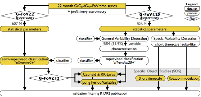
7.2.3.1 Overview
An overview of the variability processing is presented in Figure 7.1. There are two main paths: one starting from≥2 G-FoV transits (left) and one from≥20G-FoV transits (right). The former results in the published nTransits:2+ classification results, and the latter results in the published Specific Object Tables of:
vari short timescale (Section 14.3.8) and vari rotation modulation (Section 14.3.6). The published Specific Object Tables of: vari rrlyrae (Section 14.3.7), vari cepheid (Section 14.3.1), and vari long period variable(Section 14.3.5) result from a mixed feed of classification candidates from the publishednTransits:2+classifier (for sources with a minimum of 12G-FoV transits) and from the unpublished nTransits:20+classifier. The data was published from the highlighted yellow boxes for sources that passed the validation filtering.
Figure 7.2 details how the sources were cross-matched on a preliminary version of the photometry.
Figure 7.1: Gaia DR2 variability processing overview. The data products appearing in Gaia DR2 (yellow boxes) are either coming from a whole sky classification of nTransits:2+or from specific objects studies. Note that nTransits:20+classification is not published. Figure 7.2 details how the three classifiers were trained.
Figure 7.2: Gaia DR2 variability classifier training for the three classifiers in Figure 7.1. The cross-match on external catalogues was performed using a preliminary version of the photometry and astrometry. The final training of the models was performed on the published photometry (though still with preliminary astrometry) on the sources identified using the preliminary photometry.
7.2.3.2 Initial light curve pre-processing
7.2.3.2.1 Definition of observation time Observation times are expressed in units of Barycentric JD (in TCB)−2 455 197.5 days, computed as follows:
1. The observation time is converted from On-board Mission Time (OBMT) into Julian date in TCB (Temps Coordonn´ee Barycentrique).
2. A correction is applied for the light-travel time to the Solar system barycentre, resulting in Barycen- tric Julian Date (BJD).
3. Although the centroiding time accuracy of the individual CCD observations is (much) below 1 ms, the per-field-of-view observation times processed and published in Gaia DR2 are averaged over typically 9 CCD observations over a time range of about 44 sec.
Conversion from flux to magnitude In the variability pipeline, magnitudes rather than fluxes are used in the various processing modules. To convert to magnitude, the zero-point magnitudes forG,GBP,GRPprovided by CU5 in the Vega system are used (Section 5.3.6.6).
Observation filtering The variability processing includes severaloperatorsthat are applied to the ingested and reconstructed photometry. Typical time series operators perform flux to magnitude conversion, outlier removal and error cleaning on the input time series to create derived (transformed and/or filtered) time series suitable for processing by specific algorithms. Chaining of these time series operators creates a hierarchy of derived time series that is used as required by the scientific analyses while ensuring that provenance is preserved.
The following list of operators are applied in sequence to the input photometric time series, a schematic showing the hierarchy of these operators is presented in Figure 7.3:
Figure 7.3: The CU7 operator chain to transform and filter time series.
1. RemoveNaNNegativeAndZeroValuesOperator: it removes photometric transits that contain NaN, negative, or 0 flux values.
2. RemoveDuplicateObservationsOperator: it removes pairs of transits (within each Gaia band) that are too close in time (within 105 min) to be observations of the same source. Such transits can occur in bright sources for which multiple artefact detections are assigned (these are known as ‘far double detections’). Since CU7 did not have access to the flags identifying the double detections transits, this ad-hoc method was applied by which close-in-time pairs of transits were removed.
3. RemoveOneCCDFromRowAcOperator: it is designed to remove one CCD point (defined by its CCD number, between 0 and 9, 0 standing for the Sky Mapper and 1 to 9 for the Astrometric Field CCDs) from each transit ofG per-CCD data whose measurements correspond to a certain CCD row and whose across-scan (AC) coordinate is outside a certain range (minimum AC=3, maximum AC=1990). It was motivated by the fact that the photometric calibration team reported problematic flux measurements for the second Astrometric Field (AF) CCD of row 5 when AC is greater than 1200. Hence, in Gaia DR2 this operator was tailored to remove the AF2 points for transits with CCD row=5 and AC coordinate>1200.
4. GaiaFluxToMagOperator: it converts fluxes to magnitudes by using the zero-point magnitudes delivered by CU5.
5. ExtremeValueCleaning: it removes points above a specific magnitude limit. Cuts were applied at G=25,GBP=24, andGRP=22 mag.
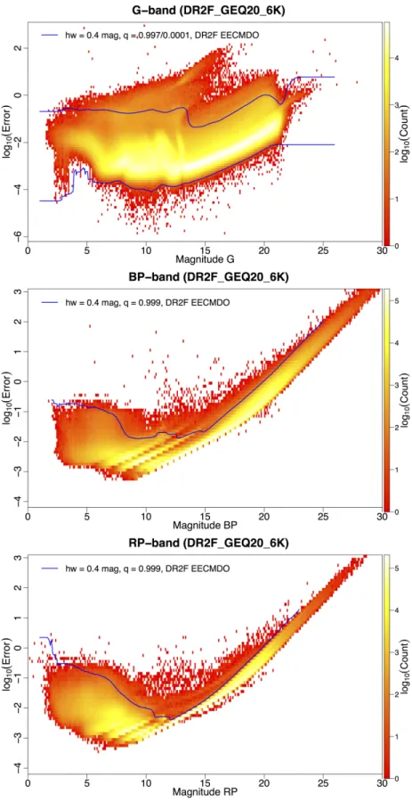
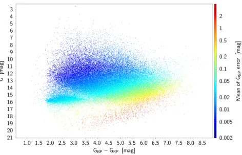
6. ExtremeErrorCleaningMagnitudeDependent: it removes individual transits above or below magnitude-dependent values. The values were determined as follows: from a sample of the CU5 photometric catalogue and for each band (limited to 6000 sources per 0.1 magnitude bin), we studied the quantile distribution of the transit magnitude errors. A decision was made to use the 99.7%
quantile for the upper value, and the 0.01% for the lower value for G data. ForGBP andGRP, a cut was applied only above the upper value of the 99.9% quantile. Figure 7.2.3.2.1 shows the distributions of the transit magnitude errors as a function of the transit magnitudes, for the 3 Gaia bands, together with the thresholds used for this operator. The latter was not applied toGper-CCD data.
7. RemoveOutliersFaintAndBrightOperator: it removes data points as follows (with configura- tion parameters described, where relevant, in the respective data product sections).
(a) A point with a too large error (intrinsically or compared to some number of times the interquar- tile range of the uncertainties) is an outlier. It is removed before the next step.
(b) Measurements at the extremes of the magnitude distribution of a time series are identified from their deviations from the median magnitude when these exceed a certain number of times the interquartile range (with different thresholds possible at the bright and faint ends). A point with an ‘extreme’ magnitude (on the faintest or brightest side, compared to the median magnitude) is an outlier unless it has similar outlying neighbours in time or projected in magnitude.
8. RemoveOutlierPerTransitOperator: it removes per-CCD outlier data points per transit. This operator only applies to per-CCD data.
9. ColorTimeSeriesOperator: it is applied to theGBPandGRPlight curves to compute theGBP−GRP
colour.
The Gaia DR2 time series are published in a Virtual Observatory table linked ingaia sourcevia the column epoch photometry url. The table includes a flag,rejected by variability, that provides information on which data points in each band were rejected by the hierarchical chain of CU7 operators up to and including RemoveOutliersFaintAndBrightOperator. Note that downstream CU7 modules may reject additional points, e.g., by applying stricter thresholds for RemoveOutliersFaintAndBrightOperator, however, such rejected points are not flagged in the Gaia DR2 archive. We mention that CU5 flags were not used in variability processing.
However they are available in the Gaia DR2 archive in columnrejected by photometryofepoch photometry url (see also Section 14.3.9).
Published output See Gaia DR2 VO Table linked in columnepoch photometry urlof tablegaia source.
7.2.3.3 Statistical parameter computation
Input All cleaned time series (Section 7.2.3.2.1) in magnitude with at least one field-of-view transit.
Method The first step in the scientific processing chain following conversion from flux to magnitude and basic cleaning (Section 7.2.3.2.1) is the computation of a number of basic descriptive, inferential and correlation statistics of all light curves. These statistics provide a first general overview of the data and their distributions and are used to determine whether variability is present in a time series of Gaia observations.
Descriptive statistics computed on the temporal evolution of the time series include (but are not limited to): the number of observations, time duration of the time series, mean observation time and the min/max time difference between two successive observations. Given the well defined nature of the Gaia scanning law and the angular separation between the 2 telescopes, the latter can be useful in identifying transits assigned to the wrong source.
Parameters that characterise the brightness of the light curve and the associated uncertainty include measures of the min, max, range, mean, median, variance, skewness, kurtosis, point-to-point scatter, interquartile range, median absolute deviation, and the signal-to-noise ratio. Where applicable, unbiased weighted and unweighted estimators as well as robust estimates are computed and compared, as they can be useful in identifying outliers, transits assigned to the wrong source or signatures of variability.
Several inferential test statistics are computed on the time series including the Kolmogorov-Smirnov (K-S) test for equality of continuous distributions, (Kolmogorov 1933; Smirnov 1939), the Ljung-Box test for randomness, (Ljung & Box 1978), the Abbe hypothesis test, (von Neumann 1941, 1942) as well as the chi-squared and Stetson test statistics, (Stetson 1996). These measures are used in the classification of a time series as either constant or variable. Only unbiased, unweighted and robust quantities are available for all Gaia DR2 time series in the Gaia catalogue.
Correlation statistics between all pairs of the three photometric bands are computed for use in the detection of general and special variability (Section 7.2.3.4). Stetson, Pearson and Spearman correlation statistics are com- puted on all permutations of pairs of the three photometric bands,G,GBP andGRP. Computation of the Stetson correlation requires that observations in each band are paired. As each band may have a different number of FoV transits, correct pairing of observations between bands is done by requiring that their time difference is less than 0.05 days. This ensures that paired observations in each band were observed in the same transit. For the Pearson and Spearman correlation statistics, the time series are filtered to remove unpaired observations. The correlation is hence performed on time series of equal length and containing only paired observations.
Run-time configuration parameters The variance, skewness and kurtosis, including weighted, unweighted and robust versions, were all computed with a sample-size bias correction.
Published output See Gaia DR2 table:vari time series statistics.
7.2.3.4 Variability Detection
Description of general and special variability detection strategies.
Input Variability analyses was only performed on field-of-view averaged photometry inG,GBP, andGRPbands.
Method In this data release, General Variability Detection (GVD) employed a supervised classifier trained on a set of identified constants and variables. Variable objects were selected from sources of different variability types derived from the crossmatch with a large number of literature catalogues (Section 7.3.3.2); they included 14 769 sources which covered most of the range of magnitudes of the data in Gaia DR2. On the other hand, constant objects were limited to crossmatched sources from a few catalogues (the least varying sources in OGLE-IV at ftp://ftp.astrouw.edu.pl/ogle/ogle4/GSEP/maps/, the Hipparcos constants in ESA 1997, and the SDSS standards in Ivezi´c et al. 2007), thus they lacked representatives in a significant magnitude range (from about 10 to 15 mag in theGband). A semi-supervised approach was employed to supplement the training set with constant objects identified in a previous iteration of variable versus constant classification, filling the gap in the magnitude distribution and leading to a total sample of 14 424 constants. The selected variable and constant objects were then characterized by time series statistics as well as average photometric quantities in order to train a Random Forest classifier, which returned an estimated completeness of at least 98% and a contamination rate of up to 2%. This classifier was applied to all 826 million sources with 20 or moreG-band field-of-view transits.
A source was considered constant or variable when the highest posterior probability class referred to either ‘con- stant’ or ‘variable’, respectively.
No p-value statistics were used or analysed for GVD in this data release.
Run-time configuration parameters The minimum classification probability to consider an object as variable was set to 50%.
Published output No data from this processing step was published in Gaia DR2. The output of this step is used as input to the general classification step (see Section 7.2.3.6).
7.2.3.5 Period search and time series modelling
Input Period search and Fourier modelling were applied to cleaned (Section 7.2.3.2.1)G-band time series (ex- pressed in magnitudes as a function of time in days) with at least five FoV transits, for sources identified as variable (Section 7.2.3.4). These methods rely also on the availability of statistical parameters (Section 7.2.3.3).
Method The process of frequency (or period) search and time series modelling, referred to collectively asVari- ability Characterization, aims to characterize the variability behaviour of time series of Gaia observations using a classical Fourier decomposition approach. The model to fit is given by Equation 7.1. The Characterization pro- cess takes as input all time series identified as variable by the precedingVariability Detectionmodule (see Section 7.2.3.4). The goal is to produce, in an automated manner, the simplest and statistically most significant model of the observed variability.
The general model of variability that we fit to time series of Gaia observations is given by:
y=
Nf
X
n=1 Nh(n)
X
k=1
An,kcos(2πk fnt+ψn,k)+
Np
X
i=0
citi (7.1)
where we assume that the reference epochtref, the middle of the time series, has already been subtracted from the time points. Np ≥ 0 is the degree of the polynomial, Nf ≥ 0 is the number of detected frequencies, and Nh(n) ≥ 1 is the number of significant harmonics of frequency fn. This multi-frequency harmonic model includes a low-order polynomial trend andnfrequencies, each withkassociated harmonics.
Run-time configuration parameters
1. For frequency search:
(a) At least≥5 FoVGtransits.
(b) No de-trending applied prior to the frequency search.
(c) Frequency searched with the Least Square method.
(d) Minimum frequency: 1.5 (∆T)−1d−1with∆Tdenoting the total time span of each time series.
(e) Maximum frequency: 20 d−1.
(f) Frequency step: (10∆T)−1d−1with∆Tdenoting the total time span of each time series.
(g) Refinement of the frequency about the most significant peak was done to a granularity of 10−6d−1.
2. For modelling:
(a) The polynomial part of Equation 7.1 was limited to degree zero.
(b) Unweighted observations were used in the fit.
(c) Non-linear fitting with the Levenberg-Marquard method was applied to the parameters of the final best model.
Published output No data from this processing step is published in Gaia DR2. The results of this step are used as input to the general classification step (see Section 7.2.3.6).
7.2.3.6 Classification
Two classification paths were followed for Gaia DR2.
1. ThenTransits:2+classification aimed at covering the whole sky. The results of this classifier can be found in the Gaia archive for selected high-amplitude pulsating variable types (δScuti/SX Phoenicis stars, RR Lyrae stars, Cepheids, long period variables). This module fed also the specific object modules CEP&RRL and LPV when there were more than 12G-FoV transits, as shown in Figure 7.1. The details of this classifier are described in Section 7.3.
2. ThenTransits:20+classification made use of the period search and modelling results from the char- acterisation module. This classifier fed (as a secondary input) the specific object modules CEP&RRL and LPV, as shown in Figure 7.1. No direct output of this classification is provided in the archive.
This section describes only thenTransits:20+classification, while thenTransits:2+classification is presented in Section 7.3.
Input ThenTransits:20+classifier is trained with attributes computed from the results of the Statistical Parameter Computation module (Section 7.2.3.3), the period search and time series modelling modules (Section 7.2.3.5), and it is applied to sources selected by the Variability Detection module (Section 7.2.3.4).
Method The module produces membership probabilities for all sources with at least 20 field-of-view transits.
The membership probabilities are obtained in two stages. In the first stage, three different classifiers (Gaussian Mixtures, Bayesian Networks, and Random Forest) produce corresponding membership probabilities based on different attribute sets. In the second stage, a meta-classifier takes as input a set of classification probabilities (denoting for each source the posterior probabilities associated with different types) from the predictions of the individual classifiers to produce the final result. The meta-classifier method is again Random Forest.
Run-time configuration parameters The four classifiers (three in stage 1 and the meta-classifier) define the input attributes via an attribute mapping that transforms the output from the previous modules into suitable clas- sification attributes. The classifiers based on Gaussian Mixtures and Bayesian Networks use the following list of attributes:
1. the first detected frequency;
2. the decadic logarithm of the amplitude of the first and second harmonics of the first detected fre- quency (two separate attributes);
3. theGBP−GRP(possibly reddened) colour index;
4. the robust percentile-based skewness (as in Eyer et al. 2017);
5. the phase difference between the first two Fourier components of the first detected frequency (after setting the phase of the first term to zero);
6. the decadic logarithm ofχ2QS O/νas defined in Butler & Bloom (2011);
7. the decadic logarithm ofχ2f alse/νas defined in Butler & Bloom (2011).
The Random Forest in the first stage uses the following list of attributes:
1. the first detected frequency;
2. theGBP−GRP(possibly reddened) colour index;
3. theGBP−G(possibly reddened) colour index;
4. theG-band Stetson variability index (Stetson 1996), pairing observations within 0.1 days;
5. the reduced chi-squared statistic of theG-band time series with respect to the constant brightness model;
6. the sample-size (un)biased (un)weighted variance (two attributes) unbiased by Gaussian uncertain- ties, in theG-band time series (Rimoldini 2014);
7. the median absolute slope (in mag d−1) of theG-band time series within a sliding window of half a day;
8. the median range of theG-band time series within a sliding window of half a day;
9. the interquartile range of theG-band magnitude distribution;
10. the decadic logarithm ofχ2f alse/νas defined in Butler & Bloom (2011);
11. the sample-size biased unweighted skewness moment standardised by its variance, in theG-band time series (Rimoldini 2014).
The Random Forest meta-classifier uses as attributes the posterior probabilities for each class estimated by the stage 1 classifiers.
In all cases, the classification scheme comprises the following classes:
1. Cepheid type stars (all subtypes included);
2. RR Lyrae type stars (all subtypes included);
3. Eclipsing binaries (all subtypes included);
4. δScuti/γDoradus sources;
5. Long Period Variables (Semi-regular variables, Mira stars);
6. Quasars;
7. Other (including all other types of variability not included in the previous types).
The combined category ofδScuti/γDoradus sources is not separated (despite their different typical periods) due to the significant contamination observed because of aliasing.
Each classifier is defined by a set of parameters the specification of which is out of the scope of this documentation.
They include the number of trees in each Random Forest, their maximum depth, the number of attributes used in each node and the minimum number of instances per class at the leaf nodes; for Bayesian Networks and Gaussian Mixtures, the configuration included a multi-stage scheme used for separating the classes and the attributes used in each node; for Gaussian Mixtures, the minimum and maximum number of components was set for each class.
Published output Only thenTransits:2+classification results were published in the Gaia DR2 tables:
vari classifier definition,vari classifier class definition,vari classifier result.
7.2.3.7 Specific Object Studies
Some variable objects benefit from additional processing that takes into account the specific properties of their variability. The Specific Object Studies (SOS) component of the variability pipeline comprises a number of ded- icated modules that aim to compute attributes specific to a variability class, and subsequently publish them in the Gaia DR2 archive. Each SOS module takes as input either the list of candidates of the corresponding variability class, as provided by the classification step (see Sect. 7.2.3.6), using a probability threshold specific to each SOS module or from the selection made in the special variability module.
Details of the selection criteria, processing, and of the output data products of each SOS module are described in the respective data product sections.
Input Source selections depend on specific SOS modules and are described in the relevant data product sections.
Method Methods are described in the relevant data product sections.
Run-time configuration parameters Run-time configuration parameters are described in the relevant data prod- uct sections.
Published output See Gaia DR2 tables:vari short timescale(Section 14.3.8),vari rotation modulation (Section 14.3.6),vari rrlyrae(Section 14.3.7),vari cepheid(Section 14.3.1), andvari long period variable (Section 14.3.5).
7.2.4 Quality assessment and validation
Author(s): Leanne Guy, Laurent Eyer, Gr´egory Jevardat de Fombelle
7.2.4.1 Verification
Extensive verifications were done on the outputs of the variability processing. A set of 430 verification rules were defined and implemented. It allowed the automatic verification of each output result of each module. Such verifications rules including but not limited to range checks, cardinality, nullity conditions allowed to fix a number of bugs and filter incorrect results. On top of that, each module made supplementary verifications that are explained within each of the following sections.
7.2.4.2 Validation
Validations of period search with external catalogues, validation of general classification with respect to other surveys were done. The validations of the different published variable star catalogues are explained within each of the corresponding sections.
7.3 All-sky classification
Author(s): Lorenzo Rimoldini
The all-sky classification results are published in the Gaia DR2 tablevari classifier resultand include can- didates for almost two hundred thousand RR Lyrae stars, about one hundred fifty thousand long period variables,
more than eight thousand Cepheids and a similar number of SX Phoenicis/δScuti stars. A subset of these can- didates was further processed by subsequent modules of the CU7 pipeline (Section 7.2.3.7), such as the ones of Cepheid and RR Lyrae stars (Section 7.4) and of long period variables (Section 7.7). Other candidates were veri- fied and validated by means of comparisons with the literature and included known misclassifications, which were nevertheless not removed in order to minimise sample selection effects and maintain the distributions of parameters more homogeneous for statistical analyses. The community is expected to take this cautionary note into account when exploiting this data set.
7.3.1 Introduction
An advance publication of the first Gaia full-sky map of Cepheids, RR Lyrae stars, SX Phoenicis/δScuti stars and long period variables is provided by automated classification of all objects with at least two FoV transits in theG band. The results of this classification can be found in the Gaia DR2 archive in the classification table associated with thenTransits:2+classifier, although subsequent filtering of sources by CU3 and CU9 increased the minimum number of FoV transits to five (after taking into account also the CU7 observation filtering of the pre-processing step described in Section 7.2.3.2).
7.3.2 Properties of the input data
Machine-learning classifiers were trained with Gaia sources selected from over seven hundred fifty thousand ob- jects crossmatched with the literature, representing a large number of variability types as well as non-varying objects. The training set included about thirty-three thousand sources filtered according to their distribution in the sky, their number of FoV transits, and their median magnitudes in theGband, as described in more details in Section 7.3.3.
All sources with two or more FoV transits in theGband were processed by the classifiers. Photometric time series in theG,GBP, andGRPbands were used after the pre-processing steps described in Section 7.2.3.2 and astrometric quantities (such as parallax and proper motion) were employed without specific selections. The results of the Statistical Parameter Computation module (Section 7.2.3.3) provided additional input information which was used directly as classification attributes or in the computation thereof.
7.3.3 Processing steps
The results of all-sky classification were obtained through the following steps.
1. Crossmatch of Gaia with literature to identify objects of known classes (Section 7.3.3.2).
2. Selection of catalogues to crossmatch and their prioritisation (in case of conflictual information on the same objects).
3. Filtering of sources not satisfying simple statistics (such as colour, magnitude, literature period, amplitude, skewness, and Abbe value computed on magnitudes sorted in time as well as in phase) that are typical of class ownership, while allowing for a large range of possible distance, extinction, and reddening.
4. Resampling of sources for a more representative distribution in the sky, in the number of FoV tran- sits, and in magnitude.
5. Pipeline run of the Statistics module on time series pre-processed as described in Section 7.2.3.2.
6. Generation and selection of classification attributes (Section 7.3.3.3).
7. Training of a multi-stage classifier with optimized parameters.
8. Application of the multi-stage classifier to the Gaia data.
9. Improvement of the training set (sources and attributes) including high-confidence classifications and iterating steps 3–6 (Section 7.3.3.5).
10. Training of the improved multi-stage classifier with optimized parameters (Section 7.3.3.4).
11. Pipeline run of the Statistics and the Classification modules on time series pre-processed as described in Section 7.2.3.2.
12. Training of contamination-cleaning classifiers and their application to the results of the previous step, for RR Lyrae stars, Cepheids, and SX Phoenicis/δScuti stars (Section 7.3.3.6).
13. Definition of classification scores of the published results (Section 7.3.3.7).
14. Assessment of completeness and contamination of the published results (Section 7.3.4).
7.3.3.1 Classes
The training set included objects of the classes targeted for publication in Gaia DR2 (listed in bold) as well as other types to reduce the contamination of the published classification results. The full list of object classes, with labels (used in the rest of this section) and corresponding descriptions, follows below.
1. ACEP: Anomalous Cepheids.
2. ACV:α2Canum Venaticorum-type stars.
3. ACYG:αCygni-type stars.
4. ARRD: Anomalous double-mode RR Lyrae stars.
5. BCEP:βCephei-type stars.
6. BLAP: Blue large amplitude pulsators.
7. CEP: Classical (δ) Cepheids.
8. CONSTANT: Objects whose variations (or absence thereof) are consistent with those of constant sources (Section 7.2.3.4).
9. CV: Cataclysmic variables of unspecified type.
10. DSCT:δScuti-type stars.
11. ECL: Eclipsing binary stars.
12. ELL: Rotating ellipsoidal variable stars (in close binary systems).
13. FLARES: Magnetically active stars displaying flares.
14. GCAS:γCassiopeiae-type stars.
15. GDOR:γDoradus-type stars.
16. MIRA: Long period variable stars of theo(omicron) Ceti type (Mira).
17. OSARG: OGLE small amplitude red giant variable stars.
18. QSO: Optically variable quasi-stellar extragalactic sources.
19. ROT: Rotation modulation in solar-like stars due to magnetic activity (spots).
20. RRAB: Fundamental-mode RR Lyrae stars.
21. RRC: First-overtone RR Lyrae stars.
22. RRD: Double-mode RR Lyrae stars.
23. RS: RS Canum Venaticorum-type stars.
24. SOLARLIKE: Stars with solar-like variability induced by magnetic activity (flares, spots, and rota- tional modulation).
25. SPB: Slowly pulsating B-type stars.
26. SXARI: SX Arietis-type stars.
27. SXPHE: SX Phoenicis-type stars.
28. SR: Long period variable stars of the semiregular type.
29. T2CEP: Type-II Cepheids.
7.3.3.2 Crossmatch with literature
Training-set objects are selected from Gaia sources crossmatched with objects associated with known classes in the literature. In order to increase the reliability of crossmatch results, a set of metrics was used in the comparison of Gaia and literature sources, always including the angular separation, and whenever possible also the time- series median magnitude in theGband, theGBP−GRPcolour, as well as time series quantities characterising the amplitude of variations in theGband such as the range or standard deviation. Such metrics were combined in a multi-dimensional distance which was minimised in an iterative process in order to allow for the tuning of empirical relations between the Gaia and literature photometric quantities (affected in particular by the different bandwidth coverage and sensitivity). The best matches were projected onto planes for all combinations of crossmatch metrics to inspect the corresponding distributions and reduce the chance of mis-matches by applying thresholds to exclude dubious outliers and excessive tails of the distributions. Although this approach sacrificed completeness in some cases, it was considered appropriate for training purposes, given the large number of sources available.
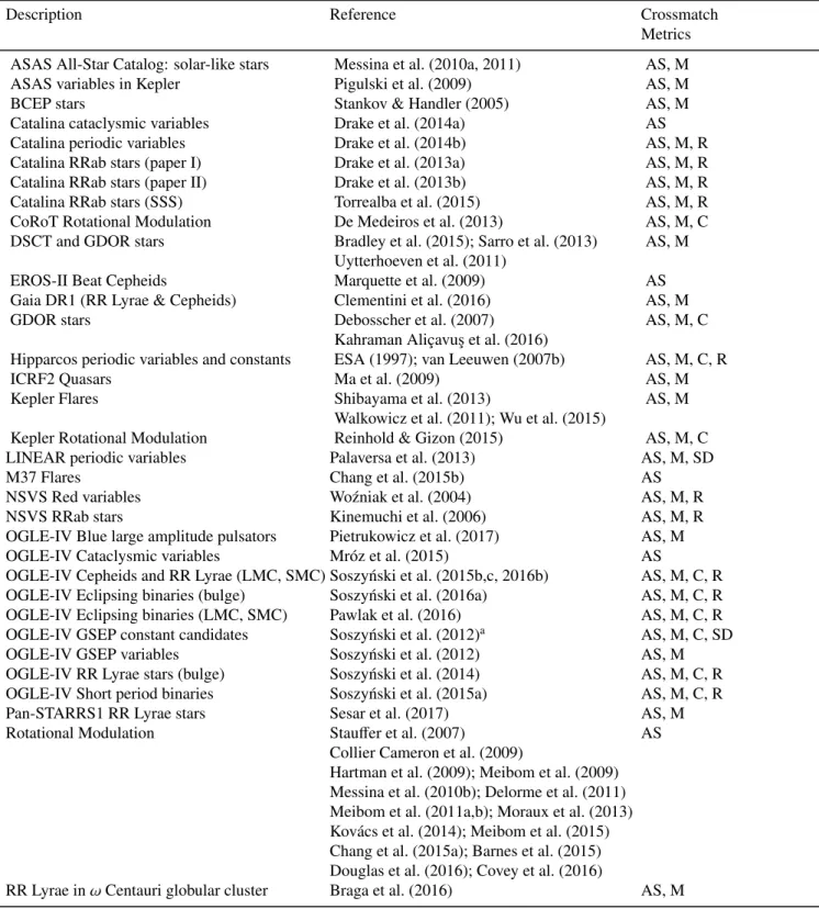
In order to sample as many regions of the sky as possible, cover most of the range of Gaia magnitudes, and include a large number of variability types, a multitude and variety of catalogues were selected from a larger set, following general reliability considerations, and prioritised in case of conflicting classifications for the same sources. The full list of catalogues employed in the training sets are presented in Table 7.1, including references and crossmatch metrics. Among the over seven hundred fifty thousand crossmatched objects available for training, only a small sample (of about 33 thousand sources) was vetted to train classifiers (Section 7.3.3.4), leaving many reliable crossmatches for the validation of results (Section 7.3.4).
Table 7.1: Crossmatch of (mostly) variable objects from the literature selected for the training set. The Table includes names of surveys and/or variability types (specified by the labels defined in Section 7.3.3.1), references, and crossmatch metrics: angular separation (AS), time-series medianG-band magnitude (M) andGBP−GRPcolour (C), time-seriesG-band magnitude range (R) and standard deviation (SD).
Description Reference Crossmatch
Metrics ASAS All-Star Catalog: solar-like stars Messina et al. (2010a, 2011) AS, M
ASAS variables in Kepler Pigulski et al. (2009) AS, M
BCEP stars Stankov & Handler (2005) AS, M
Catalina cataclysmic variables Drake et al. (2014a) AS
Catalina periodic variables Drake et al. (2014b) AS, M, R
Catalina RRab stars (paper I) Drake et al. (2013a) AS, M, R
Catalina RRab stars (paper II) Drake et al. (2013b) AS, M, R
Catalina RRab stars (SSS) Torrealba et al. (2015) AS, M, R
CoRoT Rotational Modulation De Medeiros et al. (2013) AS, M, C
DSCT and GDOR stars Bradley et al. (2015); Sarro et al. (2013) AS, M Uytterhoeven et al. (2011)
EROS-II Beat Cepheids Marquette et al. (2009) AS
Gaia DR1 (RR Lyrae & Cepheids) Clementini et al. (2016) AS, M
GDOR stars Debosscher et al. (2007) AS, M, C
Kahraman Alic¸avus¸ et al. (2016)
Hipparcos periodic variables and constants ESA (1997); van Leeuwen (2007b) AS, M, C, R
ICRF2 Quasars Ma et al. (2009) AS, M
Kepler Flares Shibayama et al. (2013) AS, M
Walkowicz et al. (2011); Wu et al. (2015)
Kepler Rotational Modulation Reinhold & Gizon (2015) AS, M, C
LINEAR periodic variables Palaversa et al. (2013) AS, M, SD
M37 Flares Chang et al. (2015b) AS
NSVS Red variables Wo´zniak et al. (2004) AS, M, R
NSVS RRab stars Kinemuchi et al. (2006) AS, M, R
OGLE-IV Blue large amplitude pulsators Pietrukowicz et al. (2017) AS, M
OGLE-IV Cataclysmic variables Mr´oz et al. (2015) AS
OGLE-IV Cepheids and RR Lyrae (LMC, SMC) Soszy´nski et al. (2015b,c, 2016b) AS, M, C, R OGLE-IV Eclipsing binaries (bulge) Soszy´nski et al. (2016a) AS, M, C, R OGLE-IV Eclipsing binaries (LMC, SMC) Pawlak et al. (2016) AS, M, C, R OGLE-IV GSEP constant candidates Soszy´nski et al. (2012)a AS, M, C, SD
OGLE-IV GSEP variables Soszy´nski et al. (2012) AS, M
OGLE-IV RR Lyrae stars (bulge) Soszy´nski et al. (2014) AS, M, C, R
OGLE-IV Short period binaries Soszy´nski et al. (2015a) AS, M, C, R
Pan-STARRS1 RR Lyrae stars Sesar et al. (2017) AS, M
Rotational Modulation Stauffer et al. (2007) AS
Collier Cameron et al. (2009)
Hartman et al. (2009); Meibom et al. (2009) Messina et al. (2010b); Delorme et al. (2011) Meibom et al. (2011a,b); Moraux et al. (2013) Kov´acs et al. (2014); Meibom et al. (2015) Chang et al. (2015a); Barnes et al. (2015) Douglas et al. (2016); Covey et al. (2016)
RR Lyrae inωCentauri globular cluster Braga et al. (2016) AS, M
Continued on next page
Table 7.1. (Continued)
Description Reference Crossmatch
Metrics
RR Lyrae in M3 Benk˝o et al. (2006) AS, M
RR Lyrae in M15 Corwin et al. (2008) AS, M
RR Lyrae in ultra-faint dwarf spheroidals Dall’Ora et al. (2006); Siegel (2006) AS, M Kuehn et al. (2008); Greco et al. (2008)
Watkins et al. (2009); Moretti et al. (2009) Musella et al. (2009, 2012)
Clementini et al. (2012); Dall’Ora et al. (2012) Boettcher et al. (2013); Garofalo et al. (2013) Sesar et al. (2014); Vivas et al. (2016)
SDSS DSCT and RR Lyrae stars S¨uveges et al. (2012) AS, M, C
SDSS-PS1-Catalina RR Lyrae stars Abbas et al. (2014) AS, M
SDSS Standard stars Ivezi´c et al. (2007) AS, M, C
Solar-like activity in the Pleiades Hartman et al. (2010) AS, M
SPB and BCEP stars Selected by Peter De Catb AS, M
SPB stars Niemczura (2003) AS, M
aSelection of the least varying sources atftp://ftp.astrouw.edu.pl/ogle/ogle4/GSEP/maps/.
bSelection of P. De Cat available athttp://www.ster.kuleuven.ac.be/˜peter/Bstars/.
7.3.3.3 Classification attributes
About one hundred fifty attributes were computed to characterise sources with photometric (and some astrometric) time series features. Each classifier (described in Section 7.3.3.4) was tested with a varying number of attributes (e.g., Guyon & Elisseeff2003) and a subset of 40 attributes represented the union of attributes used by all classifiers.
The employed classification attributes are defined below, with units quoted in brackets after the attribute name (unless the attribute is dimensionless).
1. ABBE: The Abbe value (von Neumann 1941, 1942) computed from the magnitudes of FoV transits in theGband.
2. BP MINUS RP COLOUR (mag): The possibly reddened colour index from the median magnitudes in theGBPandGRPbands.
3. BP MINUS G COLOUR (mag): The possibly reddened colour index from the median magnitudes in theGBPandGbands.
4. DENOISED UNBIASED UNWEIGHTED KURTOSIS MOMENT (mag4): The sample-size un- biased and unweighted kurtosis central moment of FoV transit magnitudes in theGband, denoised assuming Gaussian uncertainties (Rimoldini 2014).
5. DENOISED UNBIASED UNWEIGHTED VARIANCE (mag2): The sample-size unbiased and un- weighted variance of FoV transit magnitudes in theGband, denoised assuming Gaussian uncertain- ties (Rimoldini 2014).
6. DURATION (d): The duration of the time series from the first to the last FoV transit observation in theGband.
7. G MINUS RP COLOUR (mag): The possibly reddened colour index from the median magnitudes in theGandGRPbands.
8. G VS TIME IQR ABS SLOPE (mag d−1): The unweighted interquartile range of the absolute val- ues of magnitude changes per unit time between successive FoV transits in theGband.
9. G VS TIME MAX SLOPE (mag d−1): The unweighted 95th percentile of magnitude changes per unit time between successive FoV transits in theGband.
10. G VS TIME MEDIAN ABS SLOPE (mag d−1): The unweighted median of the absolute values of magnitude changes per unit time between successive FoV transits in theGband.
11. IQR BP (mag): The unweighted interquartile magnitude range of FoV transits in theGBPband.
12. IQR RP (mag): The unweighted interquartile magnitude range of FoV transits in theGRPband.
13. LOG QSO VAR: The decadic logarithm of the reduced chi-square of FoV transit magnitudes in theGband with respect to a parameterised quasar variance model, represented by log10(χ2QSO/ν) in Butler & Bloom (2011); see Rimoldini et al. (in preparation) for details on the parameter values for the Gaia data.
14. LOG NONQSO VAR: The decadic logarithm of the reduced chi-square of FoV transit magnitudes in theGbandnotto follow a parameterised quasar variance model, represented by log10(χ2False/ν) in Butler & Bloom (2011); see Rimoldini et al. (in preparation) for details on the parameter values for the Gaia data.
15. MAD G (mag): The unweighted median absolute deviation from the median magnitude of FoV transits in theGband.
16. MAX ABS SLOPE HALFDAY (mag d−1): The maximum value of the magnitude ranges of FoV transits in theGband within sliding windows of half a day, divided by the time span of theG-band observations within such sliding windows.
17. MEAN G (mag): The unweighted arithmetic mean magnitude of FoV transits in theGband.
18. MEAN BP (mag): The unweighted arithmetic mean magnitude of FoV transits in theGBPband.
19. MEAN RP (mag): The unweighted arithmetic mean magnitude of FoV transits in theGRPband.
20. MEDIAN ABS SLOPE HALFDAY (mag d−1): The unweighted median of the magnitude ranges of FoV transits in theGband within sliding windows of half a day, divided by the time span of the G-band observations within such sliding windows.
21. MEDIAN ABS SLOPE ONEDAY (mag d−1): The unweighted median of the magnitude ranges of FoV transits in theGband within sliding windows of one day, divided by the time span of theG-band observations within such sliding windows.
22. MEDIAN G (mag): The unweighted median magnitude of FoV transits in theGband.
23. MEDIAN BP (mag): The unweighted median magnitude of FoV transits in theGBPband.
24. MEDIAN RANGE HALFDAY TO ALL: The unweighted median of the magnitude ranges of FoV transits in theGband within sliding windows of half a day, divided by theG-band magnitude range of the full time series.
25. MEDIAN RP (mag): The unweighted median magnitude of FoV transits in theGRPband.
26. NONQSO PROB: A quantity distributed according to the null-hypothesis distribution ofχ2QSO, given the data, for non-quasar objects, computed from a parameterised quasar variance model with magni- tudes of FoV transits in theGband, related toP(χ2QSO|x,not quasar) in Butler & Bloom (2011); see Rimoldini et al. (in preparation) for details on the parameter values for the Gaia data.
27. NORMALISED CHI SQUARE EXCESS: The difference between the chi-square of FoV transit magnitudes in theGband and the mean of the chi-square distribution expected for constant objects (i.e., the number of degrees of freedom), normalised by the standard deviation of the chi-square distribution of constant objects (i.e., the square root of twice the number of degrees of freedom).
28. OUTLIER MEDIAN G: The absolute difference between the most outlying FoV transit magnitude with respect to the median magnitude in theG band, normalised by the uncertainty of the most outlying measurement.
29. PARALLAX (mas): The parallax value of the source derived from a preliminary astrometric solution (Section 7.2.2.1).
30. PROPER MOTION (mas yr−1): The proper motion of the source projected in the sky derived from a preliminary astrometric solution (Section 7.2.2.1).
31. PROPER MOTION ERROR TO VALUE RATIO: The ratio between the estimated projected proper motion uncertainty and the projected proper motion value of the source, derived from a preliminary astrometric solution (Section 7.2.2.1).
32. RANGE G (mag): The magnitude range of FoV transits in theGband.
33. REDUCED CHI2 G: The reduced chi-square of FoV transit magnitudes in theGband.
34. SIGNAL TO NOISE STDEV OVER RMSERR G: The ratio between the sample-size biased un- weighted standard deviation of FoV transit magnitudes in theGband and the root-mean-square of their uncertainties.
35. SKEWNESS G: The sample-size unbiased and unweighted skewness central moment of FoV transit magnitudes in theG band, normalised by the third power of the unbiased unweighted standard deviation of the same time-series measurements.
36. SKEWNESS PERCENTILE 5: A robust measure of the skewness of the magnitude distribution of FoV transits in theGband, computed as (P95+P5−2P50)/(P95−P5) wherePnis thenth unweighted percentile.
37. STETSON G: The single-band Stetson variability index (Stetson 1996) computed from the magni- tudes of FoV transits in theGband, pairing observations within 0.1 days.
38. STETSON G BP: The double-band Stetson variability index (Stetson 1996) computed from the magnitudes of FoV transits in theGandGBPbands, pairing observations in different bands within 0.001 days.
39. TRIMMED RANGE G (mag): The magnitude range between the 5th and 95th unweighted per- centiles of FoV transits in theGband.
40. TRIMMED RANGE RP (mag): The magnitude range between the 5th and 95th unweighted per- centiles of FoV transits in theGRPband.
7.3.3.4 Classification models
A hierarchical structure of Random Forest (Breiman 2001) classifiers identified objects in progressively more detailed (groups of) classes. For Gaia DR2, we focused on high-amplitude variable stars, so objects with negligible or low amplitude variations were first separated from the high amplitude ones, which were then split into the types and subtypes of interest by subsequent classifiers.
Every Random Forest classifier was configured with unlimited depths and with a minimum number of instances per class at the leafs set to one. Other configuration parameters (number of treesnTreeand number of tested attributesmTryto best split the data at a given node of a tree), the training-set classes to identify (specified by the labels defined in Section 7.3.3.1), and the selected attributes (described in Section 7.3.3.3) are listed below for each classifier. Aggregations of types are denoted by connecting single type labels with an underscore (unless indicated otherwise in brackets).
1. Random Forest classifier configured withnTree=400 andmTry=10.
(a) Training set:
i. 14 684 CONSTANT;
ii. 3885 LOW AMPLITUDE VARIABLE (ACV, ACYG, BCEP, low-amplitude DSCT GDOR, ELL, FLARES, GCAS, GDOR, OSARG, ROT, SOLAR LIKE, SPB, SXARI);
iii. 14 999 OTHER VARIABLE (ACEP, ARRD, BLAP, CEP, CV, DSCT, ECL, MIRA, QSO, RRAB, RRC, RRD, RS, SR, SXPHE, T2CEP).
(b) Attributes: BP MINUS G COLOUR, BP MINUS RP COLOUR,
DENOISED UNBIASED UNWEIGHTED VARIANCE, DURATION, G MINUS RP COLOUR, G VS TIME MEDIAN ABS SLOPE, IQR BP, IQR RP, LOG NONQSO VAR, LOG QSO VAR, MAD G, MEDIAN ABS SLOPE ONEDAY, MEDIAN BP, MEDIAN G, MEDIAN RP,
NONQSO PROB, NORMALISED CHI SQUARE EXCESS, OUTLIER MEDIAN G, RANGE G, REDUCED CHI2 G, SIGNAL TO NOISE STDEV OVER RMSERR G, SKEWNESS PERCENTILE 5, STETSON G, STETSON G BP, and TRIMMED RANGE RP.
2. Random Forest classifier configured withnTree=321 andmTry=4 (not relevant to the classification results published in Gaia DR2, but still described for details on the objects of low-amplitude types employed).
(a) Training set:
i. 363 ACV ACYG BCEP GCAS SPB SXARI (combination of poorly represented low- amplitude objects characterized by multiperiodic, pulsating, rotating, or irregular light variations);
ii. 866 DSCT GDOR LOW AMPLITUDE (DSCT, GDOR, and DSCT-GDOR hybrids with low amplitude variations);
iii. 397 ELL;
iv. 996 OSARG;
v. 1247 SOLARLIKE FLARES ROT.
(b) Attributes: BP MINUS RP COLOUR, DURATION, G MINUS RP COLOUR, IQR RP, LOG QSO VAR, MEAN BP, MEAN G, PARALLAX, PROPER MOTION.
3. Random Forest classifier configured withnTree=336 andmTry=3.
(a) Training set: 10 BLAP, 711 CEP ACEP T2CEP, 518 CV, 1326 DSCT SXPHE, 3861 ECL, 1945 MIRA SR, 1996 QSO, 4108 RRAB RRC RRD ARRD, and 500 RS.
(b) Attributes: ABBE, BP MINUS RP COLOUR,
DENOISED UNBIASED UNWEIGHTED VARIANCE, G MINUS RP COLOUR, G VS TIME MAX SLOPE, MEAN G, MEAN RP, MEDIAN ABS SLOPE ONEDAY, MEDIAN RANGE HALFDAY TO ALL, NORMALISED CHI SQUARE EXCESS, PARALLAX, PROPER MOTION, PROPER MOTION ERROR TO VALUE RATIO, RANGE G, and SKEWNESS G.
4. Random Forest classifier configured withnTree=202 andmTry=3.
(a) Training set: 2922 RRAB, 969 RRC, 197 RRD, and 20 ARRD.
(b) Attributes: BP MINUS RP COLOUR,
DENOISED UNBIASED UNWEIGHTED KURTOSIS MOMENT, G VS TIME IQR ABS SLOPE, G VS TIME MAX SLOPE,
NORMALISED CHI SQUARE EXCESS, STETSON G, and TRIMMED RANGE G.
5. Random Forest classifier configured withnTree=135 andmTry=3.
(a) Training set: 99 ACEP, 455 CEP, and 157 T2CEP.
(b) Attributes: BP MINUS RP COLOUR, DURATION, LOG NONQSO VAR, LOG QSO VAR, MAX ABS SLOPE HALFDAY, MEAN G,
MEDIAN ABS SLOPE HALFDAY, and MEDIAN RP.
7.3.3.5 Semi-supervised classification
Semi-supervised classification was applied to constant objects, RR Lyrae stars, and long period variables, in order to improve their representation in the training set as follows.
1. High-confidence classifications of such classes were selected as candidate training sources.
2. Candidate training objects were filtered by the statistics mentioned in item 3 of Section 7.3.3, except for the literature period and the Abbe value computed on phase-sorted magnitudes (not available for results classified without period computation).
3. Filtered candidate training objects were selected to cover regions in the sky and/or magnitude inter- vals that lacked proper representation in the training set.
7.3.3.6 Contamination cleaning
The contamination of preliminary classification results was reduced with the help of dedicated classifiers applied to RR Lyrae stars, Cepheids, and SX Phoenicis/δScuti stars, separately for each type, as follows.
1. Samples of true positives and false positives (according to crossmatched objects) were selected from the candidates of the previous classification stage.
2. Classification attributes were generated and selected.
3. A binary classifier of true positives versus false positives (in similar amounts) was trained and opti- mized.
4. The preliminary classification candidates (above some minimal level of classification probability depending on the type) were processed by the binary classifier (item 3) and objects classified as true positives with a minimum probability of 50 per cent were retained.
7.3.3.7 Classification score
The results of the contamination-cleaning classifiers are associated with classification scores which express the confidence of the classifier given the training set, thus such scores should not be interpreted as true probabilities.
The scores of Gaia DR2 classification results are obtained by linearly mapping the internal classifier probabilities to values within a range from zero to one (from the weakest to the strongest candidate), for each variability type.
7.3.4 Quality assessment and validation
Author(s): L´aszl´o Moln´ar, Emese Plachy, ´Aron Juh´asz, Lorenzo Rimoldini
The verification of results and their validation are performed by employing:
1. SOS of Cepheids and RR Lyrae stars applied to sources with at least 12 FoV measurements in theG band (Section 7.4).
2. SOS of long period variables applied to sources with at least 12 FoV measurements in theGband (Section 7.7).
3. The crossmatch of Cepheids and RR Lyrae star candidates with objects in the Kepler/K2 fields (Section 7.3.4.1, Section 7.3.4.2).
4. Crossmatched objects not included in the training set (Rimoldini et al., in preparation).
7.3.4.1 Verification
The verification of RR Lyrae and Cepheid candidates with Kepler/K2 fields is summarised here (for more details, see Moln´ar et al. 2018). We analysed the Gaia DR2 candidates in circular areas with a 8.5 degree radius centred on the fields of view of the original Kepler mission and the K2 mission observing Campaigns up to Field 13 (Howell et al. 2014,https://keplerscience.arc.nasa.gov/k2-fields.html). The prime Kepler mission observed a single field of view towards Lyra-Cygnus for four years. The K2 mission is ordered into campaigns along the Ecliptic; one campaign lasts for 60–80 days and then the spacecraft is reoriented. The Gaia DR2 candidates in these fields were crossmatched with the Kepler Input Catalog (KIC), the K2 Ecliptic Plane Input Catalog (EPIC), and the list of K2 targets selected for observation (Brown et al. 2011; Huber et al. 2016). The resolution of Kepler (400pixel−1) is much poorer than the one of Gaia, leading to some ambiguity in crossmatching the Gaia sources with the K2 targets. Nevertheless, RR Lyrae and Cepheid variations can be recovered even if the target is blended with another star within the photometric aperture of Kepler. We found no cases where two or more RR Lyrae or Cepheid candidates from Gaia would fall into the same aperture. We did not crossmatch sources from Campaign 9 that targeted the Galactic Bulge as the high source number density and the limited resolution of Kepler lead to strong confusion and data from OGLE was deemed superior to that of Kepler in this region.
We also made a list of known or suspected RR Lyrae stars that were proposed for observation and confirmed by Kepler, so that the completeness of Gaia DR2 candidates could be assessed from the rate of missed identifications.
7.3.4.2 Validation
The validation of RR Lyrae and Cepheid candidates with Kepler/K2 fields is summarised here (for more details, see Moln´ar et al. 2018). For the Lyra-Cygnus field, we visually inspected the Simple Aperture Photometry (SAP) and Pre-search Data Conditioning (PDC) SAP light curves of each target that was selected for observation in at least one observing quarter (one three-month segment of the original mission). We identified 48 RR Lyrae stars from the Gaia DR2 candidates, four of which were found not to be of the RR Lyrae type. Twelve other known RR Lyrae stars were not among the Gaia DR2 candidates, suggesting a sample completeness of about 78 per cent.
The original Kepler mission also acquired 52 Full-Frame Images (FFI). We extracted light curves for the objects not targeted by the mission from these images using the f3code (Montet et al. 2017). We compared the light curves folded with the fundamental periods derived from the Gaia data as well as from the FFI data visually.
Out of the 267 additional stars from the Gaia DR2 RR Lyrae candidates, we were able to classify 185 as RRAB or RRC variables (the other ones were either not RR Lyrae stars or associated with unreliable photometry). The combination of this set and the 48 stars described in the previous paragraph suggests a purity of the sample of at least 75 per cent.
In the K2 fields, we checked the light curves available for the targeted stars. These include the SAP/PDCSAP data sets provided by the mission as well as the available community-created light curves for selected campaigns. Out of the 1395 RR Lyrae candidates with counterparts in the K2 fields, 1371 were classified as RRAB or RRC in Gaia DR2, while 24 candidates turned out not to be RR Lyrae variables. The confirmed candidates are part of a larger set of 1816 known RR Lyrae stars in the K2 fields, suggesting a completeness rate around 75 per cent, in agreement with the one estimated from the original Kepler field, and a purity of 98 per cent (with a worst-case lower limit of 51 per cent) for the Ecliptic fields outside the Bulge. The interpretation of the purity value, however, is complicated by the biases in the selection of various targets for the K2 mission. About the classification of RR Lyrae stars into subclasses, 31 of the 1371 confirmed candidates were associated with the incorrect subtype, with misclassification rates of 1, 9, and 50 per cent for RRAB, RRC, and RRD types, respectively.
Cepheids were very sparse in the original Kepler fields. Among the Gaia DR2 Cepheid candidates, we found 38 Cepheid-type stars (ACEP, CEP, T2CEP) in the K2 fields and we were able to confirm 22, and assume 3 more of them (about 66 per cent). In the original field, we confirm the detection of the classical Cepheid V1154 Cyg and the T2CEP HP Lyr, while the semi regular star V677 Lyr was misclassified as T2CEP. However, the low number of targets prevented us from drawing more detailed conclusions.
7.4 Cepheid and RR Lyrae stars
Author(s): Gisella Clementini, Vincenzo Ripepi, Roberto Molinaro
We validate and refine the detection and classification of all-sky candidate RR Lyrae and Cepheid variables pro- vided by the general variable star analysis pipeline from about 22 months of GaiaG,GBP,GRPphotometry.
7.4.1 Introduction
We produce a list of confirmed all-sky RR Lyrae and Cepheid stars cleaned from contaminating objects and other types of variables falling into the same period domain. For all stars we provide a number of attributes (with related errors) to be published in the second Gaia Data Release among which, specifically: period, peak-to-peak amplitudes, mean magnitudes and epoch of maximum light inG,GBP,GRPbands (whenGBPandGRPare available)
as well as Fourier parameters from theG-band light curves. Additionally, for RR Lyrae stars for which theφ31
Fourier parameter is available we provide a metallicity ([Fe/H]) estimate and, for RRab types we also publish an estimate of the interstellar absorption in theG-band. Also, for Cepheid stars with period shorter than about 6 days we provide an estimate of metallicity ([Fe/H]).
7.4.2 Properties of the input data
Selection criteria:
• sources classified as candidate Cepheid and RR Lyrae variables from the Classifiers;
• a minimum number of 12G-FoV transits, before applying an outlier removal procedure specifically tailored to Cepheids and RR Lyrae stars to discard obvious wrong epoch data;
• a peak-to-peak amplitude>0.1 mag in theG-band;
• periods in the range of 0.2-1.0 days for the RR Lyrae variables.
7.4.3 Calibration models
The SOS Cep&RRL processing uses tools such as: period-amplitude (PA) and period-luminosity (PL) relations in theG-band, as described in the documentation for the processing of RR Lyrae and Cepheid stars released in Gaia Data Release 1, (Clementini et al. 2016). For the Gaia Data Release 2 data processing (Clementini et al. 2018) we also use tools based on theGBPandGRPphotometry, such as the period-luminosity in the RP-band and the period-Wesenheit (PW) relation inG,GRP. Furthermore, we implemented i) use of parallaxes according to the Astrometric Based Luminosity formulation, (i.e. working directly in parallax space; see, e.g., (Gaia Collaboration et al. 2017) and references therein) and applying different PL, PW relations depending on source position on sky (whether in the Large Magellanic Cloud, in the Small Magellanic Cloud or outside them); ii) calculation of metallicity ([Fe/H]) for the RR Lyrae stars and for δCepheid variables with period shorter than about 6 days from the Fourier parameters and, iii) calculation of interstellar absorption in theG-band for the RRab stars from a relation based onG-band peak-to-peak amplitude and period.
7.4.4 Processing steps
The processing includes the following steps common to both RR Lyrae and Cepheid stars (see Fig. 1 in Clementini et al. 2018):
1. Derivation of period and harmonics (amplitudes and phases) by non-linear Fourier analysis, 2. Measurement of light curve parameters (mean magnitudes, amplitudes, epochs of maximum light,
etc.),
3. Consistency check of the periods derived from the 3 bands (G,GBP,GRP), 4. Search for secondary periodicities.
The following additional steps are then applied to sources confirmed as RR Lyrae stars (see Fig. 2 in Clementini et al. 2018):
1. RR Lyrae Double-mode search, 2. Non-linear double-mode modelling, 3. Amplitude ratios,
4. Mode identification,
5. RR Lyrae Classification and validation, 6. Stellar parameters derivation: metallicity,
7. Stellar parameters derivation: absorption in theG-band for RRab stars.
and the following additional steps applied to sources confirmed as Cepheid variables (see Fig. 3 in Clementini et al.
2018):
1. Cepheid Multimode search, 2. Cepheid Type identification, 3. Type II Cepheid Subclassification, 4. δCepheid Mode identification, 5. ACEP Mode identification,
6. Cepheid Classification and validation,
7. Stellar parameters derivation: metallicity forδCepheid variables with period shorter than about 6 days.
7.4.5 Quality assessment and validation
Quality assessment and validation of the results are performed by crossmatching with catalogues of known RR Lyrae and Cepheid stars from other surveys (OGLE, Catalina, Linear, catalogues of variable stars in globular clusters and dwarf spheroidal galaxies).
7.4.5.1 Verification
Verification is done by crossmatching with catalogues of known RR Lyrae stars and Cepheid stars and comparing source attributes computed by SOS Cep&RRL with those published by OGLE in particular.
7.4.5.2 Validation
Taking advantage of the comparison between properties of RR Lyrae and Cepheid variable candidates derived by the SOS pipeline and those of known objects in the literature, we operated a selection of the candidates that led to the final published catalogue. More in detail, from the original 639 828 RR Lyrae and 72 455 Cepheid candidates, 140 784 and 9 575 objects passed this validation step.
7.5 Solar-Like variables
Author(s): Elisa Distefano, Alessandro Lanzafame, Leanne Guy
The Gaia DR2 provides a list of 147 535 solar-like variable star candidates obtained by the analysis of about 22 months of Gaia photometry. For each of these candidates, the Release supplies different parameters like the stellar rotation period, the amplitude of variability and a list of photometric outliers that could be possible flare events candidates. This section describes the methods and algorithms used for obtaining this list, as well as the verification and validation performed on the obtained sample. All the details on the solar-like analysis methods and results are extensively described in Lanzafame et al. (2018).
7.5.1 Introduction
Solar-like stars are characterised by variability phenomena due to a solar-like magnetic activity that occurs in all the main sequence stars with a spectral type later the F5. The most important variability phenomena exhibited by solar-like stars are the rotational modulation of the stellar flux and the occurrence of flare events. The rotational modulation of the stellar flux is due to the dark spots and bright faculae unevenly distributed over the stellar disk.
The stellar rotation modulate the visibility of such surface inhomogeneities and consequently the flux coming from the star. Hence, the period of light curves, for these stars, is coincident with the stellar rotation period. Flare events are sporadic outbursts due to reconnection of magnetic fields with subsequent plasma heating, particles acceleration and emission in several bands, particularly UV and X-rays. A description of solar-like variability phenomena can be found in Distefano et al. (2012) and references therein. The detection and characterisation of solar-like stars is performed by means of the SVD-Solar-Like and the SOS-Rotational-Modulation packages. The first package has the tasks to perform a first selection of solar-like candidates and to identify photometric outliers. The SOS package has the task to detect and characterise rotational-modulation variability on the solar-like candidates.
7.5.2 Properties of the input data
The input sources processed by the SVD-Solar-Like-SOS-Rotational-Modulation pipeline were selected from the catalogue of sources having at least 20 observations in theG band. From this catalogue, we selected the main sequence stars with a spectral type later then F5. This selection has been done by looking at the position of the stars in theMGvs.GBP−GRPdiagram, and therfore the parallax of the star is needed. In order to limit the errors on theMGcomputation, we selected only stars with a relative error in parallax less than 20%. A second criterion used to select the input stars is based on the time sampling ofGobservations. As described in Distefano et al. (2012), the analysis of solar-like variables requires that theGand theGBP−GRPtime-series can be segmented in small sub- series. The SVD-Solar-Like-SOS-Rotational-Modulation pipeline was employed to process only sources whose time-series can be split in at least two segments with a number of observationsNG ≥ 12. See Lanzafame et al.
(2018) for more details on the selection procedure.
7.5.3 Processing steps
The main processing steps of the SVD-Solar-Like-SOS-Rotational-Modulation pipeline are the following:
• selection of the input sources