Cloud Use Cases

(1)

Cloud Use Cases

Andras Markus², Andre Marques¹, Gabor Kecskemeti¹, and Attila Kertesz²⁽B⁾

1 Liverpool John Moores University, Liverpool, UK g.kecskemeti@ljmu.ac.uk

2 University of Szeged, Szeged, Hungary keratt@inf.u-szeged.hu

Abstract. In the paradigm of Internet of Things (IoT), sensors, actuators and smart devices are connected to the Internet. Application providers utilize the connectivity of these devices with novel approaches involving cloud computing. Some applications require in depth analysis of the interaction between IoT devices and clouds. Research in this area is facing questions like how we should govern such large cohort of devices, which may easily go up often to tens of thousands. In this chapter we investigate IoT Cloud use cases, and derive a general IoT use case. Dis- tributed systems simulators could help in such analysis, but they are problematic to apply in this newly emerging domain, since most of them are either too detailed, or not extensible enough to support the to be modelled devices. Therefore we also show how generic IoT sensors could be modelled in a state of the art simulator using our generalized case to exemplify how the fundamental properties of IoT entities can be represented in the simulator. Finally, we validate the applicability of the introduced IoT extension with a ﬁtness and a meteorological use case.

Keywords: Internet of Things

·

Cloud computing

·

^Simulation

1 Introduction

The Internet of Things (IoT) groups connected sensors (e.g. heart rate, heat, motion, etc.) and actuators (e.g. motors, lighting devices) allowing for automated and customisable systems to be utilised [8]. IoT systems are currently expanding rapidly as the amount of smart devices (sensors with networking capabilities) is growing substantially, while the costs of sensors decreases.

IoT solutions are often used a lot within businesses to increase the performance in certain areas and allow for smarter decisions to be made based on more accurate and valuable data. Businesses have grown to require IoT systems to be accurate as decisions based on their data is relied on heavily. An example of IoT in industry is the tracking of parcels for delivery services. The system can provide users with real time information of where their parcel currently is and notify them of potential arrival times. This requires a large infrastructure to facilitate as there is a lot of data being produced.

c The Author(s) 2018

I. Ganchev et al. (Eds.): Autonomous Control for a Reliable Internet of Services, LNCS 10768, pp. 313–336, 2018.

https://doi.org/10.1007/978-3-319-90415-3_12

(2)

Many sensors have different behaviour. For example, a heart rate sensor has different behaviour to a light sensor in that a heart rate sensor relies on human behaviour which is inheritably unpredictable, whereas a light sensor could be predicted quite accurately based on the time of day/location. Predicting how a sensor may impact a system is important as companies generally want to leverage the most out of an IoT system however an incorrect estimation of the performance impact can damage the performance of other systems (e.g. using too many sensors could flood the network, potentially causing inaccurate data, slow responses, or system crashes). As there are many ways a sensor can behave it is difficult to predict the impact they may have on a scalable system, therefore they must be tested to determine what the system can handle. Performing this testing could be costly, time consuming, and high risk if the infrastructure has to be created and a wide range of sensors are purchased before any information is obtained about the system. It is even more difficult to determine the impact of a prototype system on the network as there may limited or no physical sensors to perform tests with. An example of this is the introduction of soil moisture sensors that analyse soil in real time and adjust water sprinklers to ensure crops have the correct conditions to grow. In order to test this IoT system effectively, a lot of these sensors are required, however they can become quite costly and difficult to implement.

There are cloud simulators that provide the tools required to perform a customised simulation of an IoT system which can somewhat accurately simulate the performance impact that a particular setup may have on an infrastructure.

The issue with simulators is that due to the wide range of sensor behaviours, to be useful to a wide range of people the simulators cannot be too speciﬁc and instead rely on extensions to be implemented in order to function. This requires a lot of specialised code (Such as the sensor’s behaviour and the network infrastructure) to be implemented on top of the chosen simulator which can take a lot of time and may have to be altered frequently when situations change. This limits the simulators application as it demands programming skills, a lot of time, and a ﬁrm understanding of the API.

In this research work we develop extensions for the DISSECT-CF [5] simulator, which already has the ability to model cloud systems, and has the potential to provide accurate representation of IoT systems. Therefore the goal of this research is to: (i) investigate IoT Cloud use cases, and (ii) derive a general IoT use case. We also show (iii) how generic IoT sensors could be modelled in a state of the art simulator using our generalized case to exemplify how the fundamental properties of IoT entities can be represented in the simulator. Finally, we (iv) validate the applicability of the introduced IoT extension with a ﬁtness and a meteorological use case.

The remainder of this paper is as follows: Sect.2presents related work, and in Sect.3, we detail our proposal for a general use case. In Sects.5and4we discuss two concrete applications, and the contributions are summarised in Sect.6.

(3)

2 Related Work

There are many simulators available to examine distributed and speciﬁcally cloud systems. These existing simulators are mostly general network simulators, e.g.

Qualnet [1] and OMNeT++ [14]. With these tools IoT-related processes can be examined such as device placement planning and network interference. The OMNeT++ discrete event simulation environment [14] is one of these examples, and it can be used in numerous domains from queuing network simulations to wireless and ad-hoc network simulations, from business process simulation to peer-to-peer network, optical switch and storage area network simulations.

There are more speciﬁc IoT simulators, which are closer to our approach. As an example, Han et al. [4] have designed DPWSim, which is a simulation toolkit to support the development of service-oriented and event-driven IoT applications with secure web service capabilities. Its aim is to support the OASIS standard Devices Proﬁle for Web Services (DPWS) that enables the use of web services on smart and resource-constrained devices. SimIoT [13] is derived from the SimIC simulation framework [12], which provides a deeper insight into the behavior of IoT systems, and introduces several techniques that simulates the communication between an IoT sensor and the cloud, but it is limited by its compute oriented activity modeling.

Moschakis and Karatza [9] have introduced several simulation concepts to be used in IoT systems. They showed how the interfacing of the various cloud providers and IoT systems could be modeled in a simulation. They also provided a novel approach to apply IoT related workloads, where data is gathered and processed from sensors taking part in the IoT system. Unfortunately, their work do not consider actuators, and they rather focus on the behavior of cloud systems that support the processing of data originated from the IoT world. The dynamic nature of IoT systems is addressed by Silva et al. [11]. They investigate fault behaviors and introduce a fault model to these systems. Although faults are important for IoT modeling, the scalability of the introduced fault behaviors and concepts are not suﬃcient for investigating large scale systems that would beneﬁt from decentralized control mechanisms.

Khan et al. [6] introduce a novel infrastructure coordination technique that supports the use of larger scale IoT systems. They build on CloudSim [3], which can be used to model a community cloud based on residential infrastructures.

On top of CloudSim they provide customizations that are tailored for their speciﬁc home automation scenarios and therefore limit the applicability of their extensions for evaluating new IoT coordination approaches. These papers are also limited on sensors/smart objects thus not allowing to evaluate a wide range of IoT applications that are expected to rise to widespread use in the near future.

Zeng et al. [15] proposed IOTSim that supports and enables simulation of big data processing in IoT systems using the MapReduce model. They also presented a real case study that validates the eﬀectiveness of their simulator.

In the field of resource abstraction for IoT, good efforts have been made towards the description and implementation of languages and frameworks for efficient representation, annotation and processing of sensed data. The integration

(4)

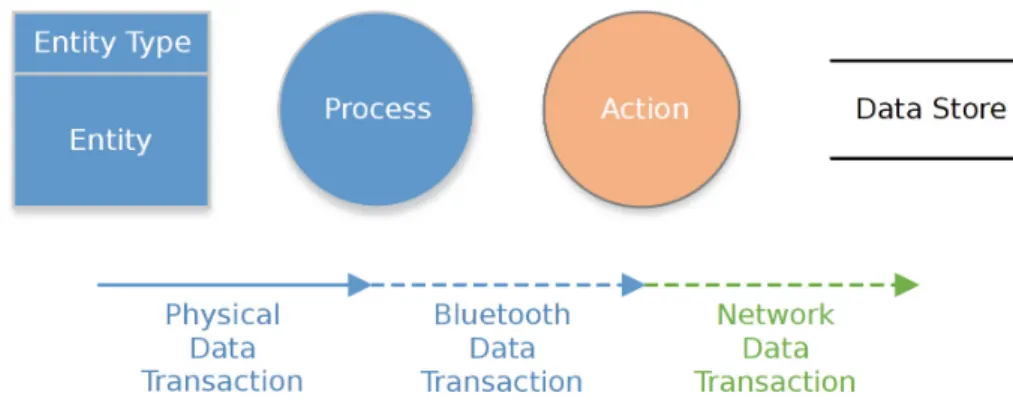
Fig. 1.Model elements of IoT use cases

of IoT and clouds has been envisioned by Botta et al. [2] by summarizing their main properties, features, underlying technologies, and open issues. A solution for merging IoT and clouds is proposed by Nastic et al. [10]. They argue that system designers and operations managers face numerous challenges to realize IoT cloud systems in practice, due to the complexity and diversity of their requirements in terms of IoT resources consumption, customization and runtime governance. We generally share these views in this work, and build on these results by specifying our own contribution in the ﬁeld of IoT Cloud simulations.

3 General IoT Extension for Cloud Simulators

The following section provides a small selection of use cases that display a wide range of behaviours, communication models, and data flows. A wide scope of use cases can provide a much better understanding of the drawbacks with current simulation solutions and will allow us to gain an insight into how we can find a common ground between them. This list is only a partial selection of possible use cases as they were selected based on the potential differences they may have, together building a fairly large pool of behavioural patterns after which intro- ducing more use cases would have had little impact on the overall experiment.

The use case ﬁgures primarily display data ﬂows (With minor context actions when necessary) as they provide an accurate enough description of the system to understand its behaviour and because simulators generally work via modelling the data transactions between entities.

In Fig.1 we introduce the basic elements of a generic IoT use case. We use these notations to represent certain properties and elements of these systems.

Next we list and deﬁne these elements:

– Entity/Entity Type. The entity box symbolises a physical device with some form of processing or communication powers. We have split the entities into 3 categories: Sensors, Gateway and Server.

(5)

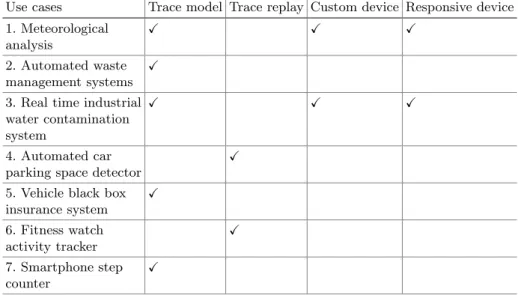
Table 1.Use case feature requirements

Use cases Trace model Trace replay Custom device Responsive device 1. Meteorological

analysis

2. Automated waste management systems

3. Real time industrial water contamination system

4. Automated car parking space detector

5. Vehicle black box

insurance system

6. Fitness watch

activity tracker

7. Smartphone step

counter

– Process. The Process circle represents some form of data processing within the linked Entity. It is used to symbolise the transformation, testing, and/or checking of data ﬂows to produce either more data ﬂows, or a contextual event to trigger. An example of this function can be the interpretation of analog input data from a sensor into something usable.

– Action. The Action circle simply represents a contextual event which generally comes in the form of a physical event. Actions usually require some form of data processing in order to trigger and thus are mostly used at the end of a data ﬂow process. An example of this is a smartphone notiﬁcation displaying a message from a cloud service.

– Data Store. The Data Store is used primarily by gateways and servers and symbolises the physical disk storage that a device might read/write to.

Although this isn’t necessary to model, it may help understand some of the diagrams as to where the data may be coming from (As sometimes the data stores are used as a buﬀer to hold the data).

– Data Transactions. Data Transactions display the movement of data between entities and processes via a range of methods. A Physical Data Transaction refers to a direct link that entities and processes may have, such as a wired connection. Alternatively Bluetooth and Network transactions are diﬀeren- tiated to assist get understanding of how links are formed (To give a small reﬂection in the distances that can be assumed. Bluetooth having a shorter range than a network transaction).

In Table1 we gathered the basic feature requirements of representative IoT use cases. We have identiﬁed 4 requirements to be supported by simulations focusing on IoT device behaviour:

(6)

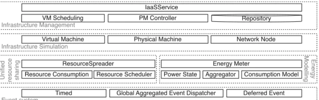
Fig. 2.The architecture of DISSECT-CF, showing the foundations for our extensions

Trace model. Allow device behaviour to be characterised by its statistical properties (e.g., distribution functions and their properties like mean, median data packet size, communication frequency etc.).

Trace replay. Let devices behave according to real-life recordings from the past. Here we expect devices to be deﬁned with pointers to trace ﬁles that contain network, storage and computing activities in a time series.

Custom device. In general, we expect that most of the simulations could be described by fulﬁlling the above two requirements. On the other hand, if the built in behaviour models are not suﬃcient, and there are no traces available, the simulation could incorporate specialised device implementations which implement the missing models.

Responsive device.We expect that some custom devices would react to the surrounding simulated environment. Thus the device model is not exclusively dependent on the internals of the device, but on the device context (e.g., having a gateway that can dynamically change its behaviour depending on the size of its monitored sensor set).

Based on these requirements, we examined seven cases ranging from smart region down to smart home applications. We chose to examine these cases by means of simulations, and we will focus on two distinguished cases further on: cases no.

1. and 6.

DISSECT-CF [5] is a compact, highly customizable open source¹ cloud simulator with special focus on the internal organization and behavior of IaaS systems. Figure2 presents its architecture. It groups the major components with dashed lines into subsystems. There are ﬁve major subsystems implemented independently, each responsible for a particular aspect of internal IaaS functionality:

(i) event system – for a primary time reference; (ii) uniﬁed resource sharing – to resolve low-level resource bottleneck situations; (iii) energy modeling – for the analysis of energy-usage patterns of individual resources (e.g., network links, CPUs) or their aggregations; (iv) infrastructure simulation – to model physical

1 Available from:https://github.com/kecskemeti/dissect-cf.

(7)

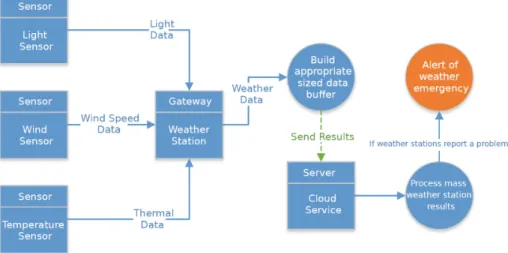
Fig. 3.1. Use case: meteorological application

and virtual machines as well as networked entities; and ﬁnally (v) infrastructure management – to provide a real life cloud like API and encapsulate cloud level scheduling.

As we aim at supporting the simulation of several thousand (or even more) devices participating in previously unforeseen IoT scenarios, or possibly existing systems that have not been examined before in more detail (e.g. in terms of scalability, responsiveness, energy eﬃciency or management costs). Since the high performance of a simulator’s resource sharing mechanism is essential, we have chosen to use the DISSECT-CF simulator, because of its uniﬁed resource sharing foundation. Building on this foundation, it is possible to implement the basic constructs of IoT systems (e.g., smart objects, sensors or actuators) and keep the performance of the past simulator.

The proposed extension provides a runnable Application interface that can take an XML file defining the Machine Data (Such as Physical Machines, Reposi- tories, and their Connection data) and an XML file defining the Simulation Data (Such as the Devices and their behaviours). The Simulation Data can contain a scalable number of Devices and each device has its own independent behaviour model defined. The behaviour of the Device can be modelled in a combination of 3 ways; a direct link to a Trace File (Which should contain the target device, timestamp, and data size), a Trace Producer Model which contains the Distribu- tion set to produce an approximation of the device trace, or finally the simulator can accept device extensions which allow custom devices to be included in the source to programmatically model more specific behaviours.

(8)

Fig. 4.6. Use case: ﬁtness tracker application

3.1 1. Use Case: Meteorological Application

In Fig.3 we reveal the typical data flow of a weather forecasting service. This application aims to make weather analysis more efficient by allowing the purchase of a small weather station kit including light sensors (to potentially capture cloud coverage), wind sensors (to collect wind speed), and temperature sensors (to capture the current ambient temperate). The weather station will then create a summary of the sensors findings over a certain period of time and report it to a Cloud service for further processing such as detecting hurricanes or heat waves in the early stages. If many of these stations are set up over a region, it can provide accurate and detailed data flow to the cloud service to produce accurate results.

In order to simulate this application, the simulator need to provide appropriate tools for performing the communications and processing, deﬁning the behaviour of the sensors and the weather station require a modelling technique to be implemented on top of the simulator (which was achieved by programming the sensors data production and the stations buﬀer reporting).

3.2 6. Use Case: Fitness Tracking Application

In Fig.4we reveal the data flow typically encountered when wearables or fitness trackers like fitbit are used. This use case aims to track and encourage the activity

(9)

of a user by collecting a wide range of data about the user (Such as current heart rate, step count, ﬂoors climbed, etc.). This data is generally collected by the wearable device and sent to the smart phone when the user accesses the smartphone applications and requests the devices to synchronise, after which the data will then be synced from the smartphone to the cloud as well, for more data processing (which could result in trophies and milestones encouraging further use of the wearable).

This provides an interesting range of behaviour as it contains a feedback mechanism to provide incentive to the user to perform speciﬁc actions based on certain circumstances. This is displayed within the Trophy and Milestone system that is implemented server side that will track certain metrics (such as average time being active daily) and provide notiﬁcations when they are reaching a goal (like a daily milestone of 1 h active per day).

This mechanism introduces an important behaviour model whereby the sensors produce data that can trigger events that indirectly change the behaviour of the sensors via a feedback loop. An example of this feedback loop can be the daily activity milestone whereby a user may perform 45 min of activity and decide to take a rest, at this point the sensors will revert back to their baseline behaviour (user is inactive therefore the sensors provide less data), however the system notiﬁes the user that only an extra 15 min is necessary to reach their milestone (the feedback), and thus the user may decide they want to hit their target and perform more activity which will then change the behaviour of the sensors yet again.

It would be difficult to simulate this case via modelling strategies as the feedback mechanism combined with the unpredictable and wide ranging human activity (most users will have different times that they are active, levels of inten- sity, and duration of exercise) have too many variables to take into consideration. There is also the consideration of the time of day being a large factor to the behaviour of the sensor, as it can be expected that the sensor will provide far less activity data during the night when the user is likely sleeping when compared to the day time. This is further compounded by time zone differences whereby if the system is used in multiple time zones it would be harder to model due to differences in when a user base may be asleep or not.

Due to the above reasons it would be required that a wide range of traces were collected in order to be able to obtain a large enough sample size of different behaviour models to run an accurate simulation of the system (which could be scaled up/down as required). This introduces problems with current simulator solutions as not only is replay functionality needed, but there must be the possibility of replaying several different traces simultaneously in order to test a system with the multitude of different behavioural models that can be expected (As there would be no point in running a simulation of a single behaviour model considering the real world application is vastly different).

(10)

4 Implementing the Extension for a Meteorological Application

Based on the generic plans discussed before, we performed the extension of the DISSECT-CF simulator towards a meteorological application covering a wider region. To derive the sensor models for the extension, we started by modelling a real-world IoT system: as one of the earliest examples of sensor networks are from the ﬁeld of meteorology and weather prediction, we choose to model the crowdsourced meteorological service of Hungary called Idokep.hu. It has been established in 2004, and it is one of the most popular websites on meteorology in Hungary. Since 2008 weather information can be viewed on Croatia and even on Germany. Detailed information of its system architecture and operation can also be found on the website: more than 400 stations send sensor data to their system (including temperature, humidity, barometric pressure, rainfall and wind properties), and the actual weather conditions are refreshed every 10 min. They also provide forecasts up to a week. They also produce and sell sensor stations capable to extend their sensor network and improve their weather predictions.

These can be bought and installed at buyer speciﬁc locations.

We followed a bottom-up approach to add IoT functionalities to the simulator, and implemented a weather prediction application using public data available on sensors and their behaviour athttp://www.idokep.hu.

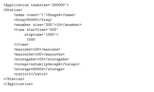
Each entity that aims to perform repeated events in DISSECT-CT has to use theTimedclass (see Fig.2), by implementing thetick()method. We added two of such classes, theApplicationand theStation. TheStationis an entity acting as a gateway. I.e., it provides the network connection for sensors, and optimises the network usage of the sensors by caching and bundling outgoing metering data of its supervised sensors. Figure5depicts how data stored about each station in an IoT system. This description is useful to set up predefined stations from files. Thetasksizeattribute of Applicationdefines the amount of data (in bytes) to be gathered in a cloud storage (sent by the stations) before their processing in a VM.

Stations have unique identiﬁers (i.e., aname). We can specify their lifetime with the tagtimeby deﬁning theirstarttimeandstoptime. The cardinality of the supervised sensor set is set viasbnumber. Alongside the set cardinality, one can also specify the average datasizeproduced by one of the sensors in the set.

To set up more stations with the same properties, one can use thecountoption in the name tag. Data generation frequency (freq) could be set for the sensor set (in milliseconds). The station’s caching mechanism is inﬂuenced with the tag ratio. This deﬁnes the amount of data to be kept at the local storage relative to the average dataset produced by the sensors at each data generation event.

If the unsent data in the local storage (which is defined instorage) overreaches the caching limit, the station is modelled to send the cached items to the cloud’s storage (identified with its network node id specified in thetorepotag). The local storage is also keeping a log of previously sent data until its capacity (defined in thestoragetag) is exceeded. The station’s network connectivity to the outside world is specified by the tagsmaxinbwandmaxoutbw.

(11)

<name count=’1’>Szeged</name>

<time starttime=’500’

stoptime=’1000’>

1000

</time>

<torepo>sztakilpdsceph</torepo>

</Station>

</Application>

Fig. 5.XML-based description of IoT systems

Individual Station entries in the XML are saved in theStationDatajava bean.

The actual data generation of the sensors is performed by theMeteringclass.

TheCloudclass can be used to specify and set up a cloud environment. This class uses DISSECT-CF’s XML based cloud loader to set up a cloud environment to be used for storing and processing data from stations. This class should also be used to deﬁne Virtual Appliances modeling the application binaries doing the in cloud processing.

The scenarios to be examined through simulations should be deﬁned by the Applicationclass. Users are expected to implement custom IoT Cloud use cases here by examining various management and processing algorithms of sensor data in VMs of a speciﬁc cloud environment. The VmCollectorclass can be used to manage such VMs, and its VmSearch()method can be used to check if there is a free VM available in the cloud to be utilized for a certain task. If this is not the case, the generateAndAdd()method can be used to deploy a new one.

4.1 Implementation with the Generic IoT Oriented Extensions The weather station’s caching behaviour is a prime example for the need of responsive device implementations. As the sensors produce data independently from each other, and they could have varying frequencies and data sizes, the station must cache all produced data before sending it to the cloud for processing. This behaviour was modelled as a custom, responsive device for which we overrode the tick()function of our new device sub-class. In DISSECT-CF terminology, this function is the one that is used to represent periodic events in the simulation,

(12)

Fig. 6.Analysis of the buﬀering behaviour in the alternative simulations of a weather station

in this particular case it was used to simulate the data reporting requests from the cloud. Each station has connections to its 8 sensors, which produced randomly sized data with the frequency of [₆₀¹−1] Hz. Upon every tick call, our custom device determines if there is a need to send its buffered contents to the cloud or not. This is based on the buffered data size that was set to be at least 1 kB before emptying the buffer.

The implementation was tested by running the original and the new implementations side-by-side so that we could analyse the network traﬃc diﬀerences.

Due to the random nature of the data production the two solutions don’t completely line up, however Fig.6 displays how the simulation extension produces a very similar result to the original implementation in that although there is a lot of randomness to the investigated scenario, the mean and median values are having a close match. The distribution is also following the same pattern:

whereby the bulk of the buﬀer loads are within 1600 bytes and are less frequent the further away from this value it goes.

At it can be observed, the basic extensions described here are mainly focusing on device behaviour. The application level operations are completely up to the user to deﬁne. E.g., application logic for how many virtual machines do we need for processing the sensor data is not to be described by the XML descriptors. In the next sub-section we will discuss such situations and explore how to combine application level behaviour with the new sensor and device models.

(13)

4.2 Evaluation with Alternative Application Level Scenarios

During our implementation and evaluation, where applicable, we used publicly available information to populate our experiments. Unfortunately, some details are unpublished (e.g. sensor data sizes, data-processing times), for those, we have provided estimates and listed them below.

In the website of Idokep.hu², we learnt that the service operates with 487 stations. Each of them has sensors at most monitoring the following environmental properties:

1. timestamp;

2. air and dew point temperature –^◦C;

3. humidity – %;

4. barometic pressure – in hPa;

5. rainfall – mm/hour and mm/day;

6. wind speed – km/h;

7. wind direction;

8. and UV-B level.

Concerning the size of such sensor data, we expect them to be save in a structured text ﬁle (eg., CSV). Stored this way, we can estimate that approximately 50 bytes (e.g., based on the website of the Murdoch University Weather Station³) are produced if each sensor produces data in every measurement.

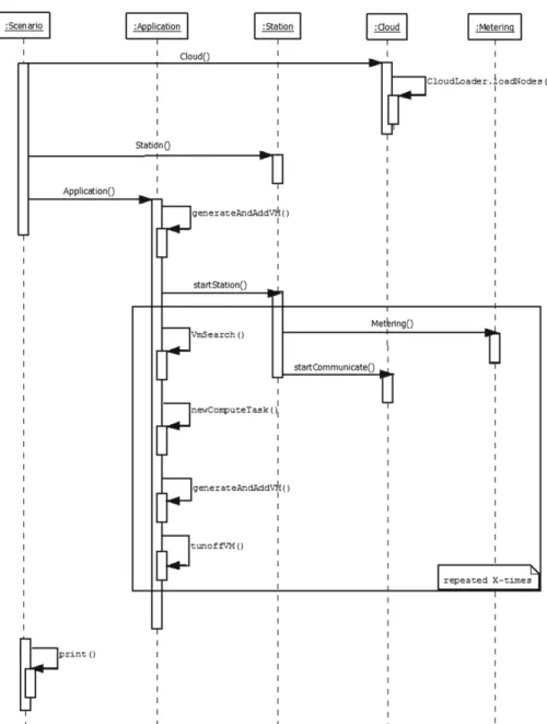
Next, we detail the steps of the behaviour of ourApplicationimplementa- tion which was used for all evaluation scenarios later (see Fig.7):

1. Set up the cloud using an XML. As we expect meteorological scenarios will often use private clouds, we used the model of our local private infrastructure (the LPDS Cloud of MTA SZTAKI);

2. Set up the 487 stations (using a scenario speciﬁc XML description) with the previously listed 8 sensors per station;

3. Start the Application to deploy an initial VM (generateAndAddVM()) for processing and to start the metering process in all stations (startStation());

4. The stations then monitor (Metering()), save and send (startCommunicate()) sensor data (to the cloud storage) according to their XML deﬁnition;

5. A daemon service checks regularly if the cloud repository received a scenario specific amount of data (see the tasksize attribute in Fig.5). If there so, then theApplication generates tasks which will finish processing within a predefined amount of time.

6. Next, for each generated task, a free VM is searched (by VmSearch()). If a VM is found, the task and the relevant data is sent to it for processing.

7. In case there are no free VMs found, the daemon initiates a new VM deploy- ment and holds back the not yet mapped tasks.

2 http://idokep.hu/automata.

3 http://wwwmet.murdoch.edu.au/downloads.

(14)

8. If at the end of the task assignment phase, there are still free VMs, they are all decommissioned (byturnoffVM()) except the last one (allowing the next rounds to start with an already available VM). Note this behaviour could be turned on/oﬀ at will.

9. Finally, theApplicationreturns to step 5.

Fig. 7.Sequence diagram of the weather station modelling use case and its relations to our DISSECT-CF extensions

(15)

4.3 Evaluation

In this sub-section, we reveal five scenarios investigating questions likely to be investigated with the help of extended DISSECT-CF. Namely, our scenarios mainly focus on how resource utilization and management patterns alter based on changing sensor behaviour (e.g., how different sensor data sizes and varying number of stations and sensors affect the operation of the simulated IoT system).

Note, the scope of these scenarios is solely focused on the validation of our proposed IoT extensions and thus the scenarios are mostly underdeveloped in terms of how a weather service would behave internally.

Before getting into the details, we clarify the common behaviour patterns, we used during all of the scenarios below. First of all, to limit simulation runtime, all of our experiments limited the station lifetimes to a single day. The start-up period of the stations were selected randomly between 0 and 20 min. The task creator daemon service of ourApplicationimplementation spawned tasks after the cloud storage received more than 250 kBs of metering data (see thetasksize of Fig.5). This step ensured the estimated processing time of 5 min/task. VMs were started for each 250 kB data set. The cloud storage was completely run empty by the daemon: the last spawned task was started with less than 250 kBs to process – scaling down its execution time. Finally, we disabled the dynamic VM decommissioning feature of the application (see step 8 in Sect.4.2).

In scenario Nô1, we varied the amount of data produced by the sensors: we set 50, 100 and 200 bytes for different cases (allowing overheads for storage, network transfer, different data formats and secure encoding etc.). We simulated the 487 stations of the weather service. Our results can be seen in Fig.8a and b. For the first case with 50 bytes of sensor data we measured 256 MBs of produced data in total, while in the second case of 100 bytes we measured 513 MBs, and in the third of 200 bytes we measured 1.02 GBs (showing linear scaling up). In the 3 cases we needed 6, 10 and 20 VMs to process all tasks respectively.

In scenario N^o2, we wanted to examine the eﬀects of varying sensor numbers and varying sensor data sizes per stations to mimic real world systems better.

Therefore, we defined a fixed case using 744 stations having 7 sensors each, producing 100 bytes of sensor data per measurement, and a random case, in which we had the 744 stations with randomly sized sensor set (ranging between 6–8) and sensor data size (50, 100 or 200 bytes/sensor). The results can be seen in Fig.9a and b. As we can see we experienced minimal differences; the random case resulted in slightly more tasks.

In scenario Nô3, we examined random sensor data generation frequencies. We set up 600 stations, and defined cases for two static frequencies (1 and 5 min), and a third case, in which we randomly set the sensing frequency between 1 and 5. In real life, the varying weather conditions may call for (or result in) such changes. In both cases, the sensors generated our previously estimated 50 bytes. The results can be seen in Fig.10a, b and c. As we can see the generated data in total: 316 MBs for 1 min frequency, 63 MBs for 5 min frequency, and 143 MBs for the randomly selected frequencies. Here we can see that the first

(16)

(a) Number of tasks (b) Evolution of tasks over time Fig. 8.Scenario N^o1

(a) Results (b) Evolution of tasks over time Fig. 9.Scenario N^o2

case required the highest number of VMs to process the sensed data, but the randomly modiﬁed sensing frequency resulted in the highest number of tasks.

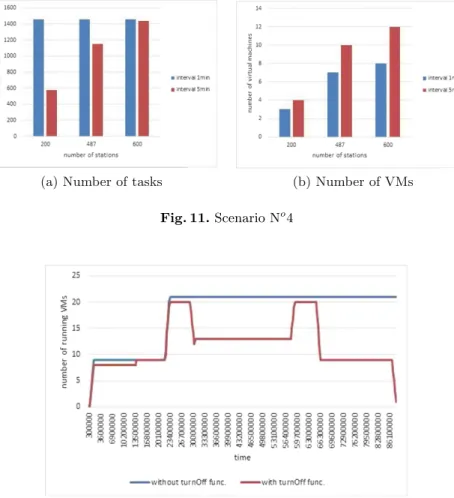
In the three scenarios executed so far the main application, responsible for processing the sensor data in the cloud, checked the repository for new transfers in every minute. In some cases we experienced that only small amount of data has arrived within this interval (i.e. task creation frequency). Therefore in scenario Nô4, we examined what happens if we widen this interval to 5 min. We executed three cases here with 200, 487 and 600 stations. The results can be seen in Fig.11a. In Fig.11b, we can read the number of VMs required for processing the tasks in the actual case. The first case has the highest difference in terms of task numbers: data coming from sensors of 200 stations needed more than 1400 tasks with 1 min interval, while less than 600 with 5 min interval. It is also interesting that with 600 stations almost the same amount of tasks were generated, but with the 5 min interval we needed more VMs to process them.

As we model a crowdsourced service, we expect to see a more dynamic behaviour regarding stations. In the previous cases we used static number of

(17)

(a) Results (b) Number of VMs

(c) Number of tasks Fig. 10.Scenario N^o3

stations per experiment, while in our final scenario, Nô5, we ensured station numbers dynamically change. Such changes may occur due to station or sensor failures, or even by sensor replacement. In this scenario we performed these changes by specific hours of the day: from 0–5 am we started 200 stations, from 6–8 am we operated 500 stations, from 9 am to 15 pm we scaled them down to 300, then from 16–18 up to 500, finally the last round from 19–24 pm we set it back to 200. In this experiment we also wanted to examine the effects of VM decommissioning, therefore we executed two different cases, one with and one without turning off unused VMs. In both cases we set the tasksize attribute to 10 kB (instead of the usual 250 kB). The results can be seen in Fig.12. We can see that without turning off the unused VMs from 6 pm we kept more than 20 VMs alive (resulting in more overprovisioning), while in the other case the number of running VMs dynamically changed to the one required by the number of tasks to be processed.

As a summary, in this section we presented ﬁve scenarios focusing on various properties of IoT systems. We have shown that with our extended simulator, we can investigate the behaviour of these systems and contribute to the development of better design and management solutions in this research ﬁeld.

(18)

(a) Number of tasks (b) Number of VMs Fig. 11.Scenario N^o4

Fig. 12.Results of scenario N^o5

5 Implementing the Extension for a Fitness Application

This use case was selected for implementation to allow us to replay real world data logs for multiple devices so that we could test the simulators trace replaying capabilities. It is important that the application can run through the trace logs for each device individually and correctly perform the network transfers that are detailed in it. The trace logs to be played were acquired with a special traffic interception application developed for the smartphone. Our application collected access and network traffic logs for the watch, smartphone, and the cloud. After data collection, the logs were saved in a file format ready to be used as an input trace to the simulator. This extension has been performed within a BSc thesis work [7] at the Liverpool John Moores University, UK.

(19)

5.1 Trace Collection

Initially, we aimed to collect all of the network traffic between the three devices with a packet analysing software (such as Wireshark) on a laptop that acted as a wireless hotspot for the smartphone. However, this severely limited the accuracy of the traces as this requires disabling the network of the fitness application, when the phone is not connected to the laptop (to ensure all its communication with the cloud is caught). On top of this, we would have lost the ability to trace the Bluetooth traffic between the watch and the smartphone.

As a result, we turned our attention of to methods that intercept network traffic directly through the phone. Despite the multitude of third party android network traffic analysers, we could not find one that met our requirements:

(i) should run at the background (allowing us to use the ﬁtness application at will); (ii) should have output logs on network and bluetooth activity either directly processable by the simulator or in a format that could be easily trans- formed to the needed form; and (iii) should remain active for long periods of time (as the log collection ran for days).

As a result, we have decided to create an application that met all of these requirements and would allow us to localise the data collection into one place.

The Fitbit connection monitor application⁴ is built on top of an android sub- system called the Xposed Framework. Using this framework, we were able to intercept socket streams for network I/O, while for bluetooth, we have used intercepted traﬃc through android’s GATT service.

A sample of intercepted data traces is shown in Fig.13. This ﬁgure shows the data that was collected from the Fitbit Connection Monitor over the course of around 2 weeks (over 20,000 trace entries of real life data). There are several interesting situations one can observe in the raw data. First, it shows peaks of network activity in cases when: (i) there was a manually invoked data synchro- nisation (ii) or when the user issued ﬁrmware update request for the watch. In contrast, there were gaps in the data collection as well. These gaps represent situations such as: (i) the user did not wear his/her watch, (ii) Bluetooth was disabled on the smartphone or (iii) the watch was not switched on (e.g., because of running out of battery power).

5.2 Implementation and IoT Extensions to DISSECT-CF

In our initial implementation, we have followed a similar approach as we did with the meteorological case. We have implemented the ﬁtness use case with the original DISSECT-CF APIs. Then we also implemented a solution that was built on top of the our new IoT oriented extensions of DISSECT-CF APIs⁵. To better understand this solution, ﬁrst we summarize the extensions.

4 The application is open source and available at https://github.com/Andrerm124/

FitbitConnectionMonitor.

5 The source code of the second implementation is available online athttps://github.

com/Andrerm124/dissect-cf/tree/FitbitSimulation.

(20)

Fig. 13.Real-life network traﬃc in the ﬁtness use case according to the long term trace collection results

Figure14presents the new extensions to DISSECT-CF. With the extension, one can define a simulation with two XML files. First, the original simulator API loads all of the physical machines from the supplied Machine XML file (the loaded up machines will represent the computational, network and storage capabilities of the IoT devices). In the second XML, device models can be linked to each of the previously loaded machines. Each model can be customised independently by altering the desired attributes of the built in device templates.

In these templates, one can deﬁne the following details: (i) machine id to bind to, (ii) time interval for the presence of the device, (iii) custom attributes and behaviour – this part still must be coded in java –, (iv) network behaviour – in the form of a trace or a distribution function, (v) typical network endpoints and (vi) data storage and caching options (both device local and remote – e.g., in the cloud). The loading of these XML ﬁles and the management of the device objects is accomplished by theApplicationclass. Finally, the extension provides alternative packet routing models as well in the form of the several implementations for theConnectionEventinterface.

(21)

Fig. 14.The IoT oriented DISSECT-CF extensions

To analyse the effectiveness of our extensions, we have compared the development time and the simulation results for the fitness application. The initial implementation has been created as custom classes for all devices participating in the use case. This required approximately 3 days of development time. In contrast, with the new extensions, barely more than 20 lines of XML code (shown in Fig.15) plus the previously collected trace files were required to define the whole simulation. To validate the new implementation, we also compared the data produced from this new and the initial completely java based implementation. We have concluded that the two implementations produced equivalent results (albeit the XML based one allowed much more rapid changes to device configurations and to their behaviour).

(22)

<?xml version="1.0" encoding="UTF-8" standalone="yes"?>

<ID>Watch</ID>

<SimulationFilePath>bluetooth_in.csv</SimulationFilePath>

</TraceFileReader>

</Device>

<ID>Smartphone</ID>

<SimulationFilePath>network_out.csv</SimulationFilePath>

</TraceFileReader>

</Device>

<ID>Cloud</ID>

<SimulationFilePath>network_in.csv</SimulationFilePath>

</TraceFileReader>

</Device>

</Devices>

</Simulation>

Fig. 15.XML model of the ﬁtness use case

5.3 Evaluation

To evaluate our extensions, we have set up the exact same situation in the simulation as we have had during the trace collection. We also ensured the simulation writes its output in terms of simulated network and computing activities in the same format as the originally collected traces. This allowed easy comparison between the simulated and the real-life traces. Figure16 show the comparison of the bluetooth trace. According to the ﬁgure, the simulation can accurately reproduce the real-life traces, i.e., the simulated data transfers occur at the pre- scribed times and have the same levels of data movement as the ones recorded in real-life. The network communication between the cloud and the smartphone has shown similar trends (thus the simulation was capable to reproduce the complete Fig.13).

(23)

Fig. 16.Watch network traﬃc comparison

6 Conclusion

Distributed systems simulators are not generic enough to be applied in newly emerging domains, such as IoT Cloud systems, which require in depth analysis of the interaction between IoT devices and clouds. Research in this area is facing questions like how we should govern such large cohort of devices, which may easily go up often to tens of thousands.

In this chapter we investigated various IoT Cloud use cases, and derived a general IoT use case. We have shown, how generic IoT sensors could be modelled in the DISSECT-CF simulator, and exempliﬁed how the fundamental properties of IoT entities can be represented. Finally, we validated the applicability of the introduced IoT extension with a ﬁtness and a meteorological application.

Acknowledgments. The research leading to these results has received funding from the European COST programme under Action identiﬁer IC1304 (ACROSS), and it was supported by the UNKP-17-4 New National Excellence Program of the Ministry of Human Capacities of Hungary. A part of this research has been performed within a BSc thesis work of A. Marques [7] at the Liverpool John Moores University, UK.

References

1. QualNet communications simulation platform.http://web.scalable-networks.com/

content/qualnet. Accessed Jan 2016

2. Botta, A., De Donato, W., Persico, V., Pescap´e, A.: On the integration of cloud computing and internet of things. In: International Conference on Future Internet of Things and Cloud (FiCloud), pp. 23–30. IEEE (2014)

3. Calheiros, R.N., Ranjan, R., Beloglazov, A., De Rose, C.A., Buyya, R.: CloudSim:

a toolkit for modeling and simulation of cloud computing environments and evaluation of resource provisioning algorithms. Softw. Pract. Experience41(1), 23–50 (2011)

(24)

4. Han, S.N., Lee, G.M., Crespi, N., Heo, K., Van Luong, N., Brut, M., Gatellier, P.:

DPWSim: a simulation toolkit for IoT applications using devices proﬁle for web services. In: IEEE World Forum on Internet of Things (WF-IoT), pp. 544–547.

IEEE (2014)

5. Kecskemeti, G.: DISSECT-CF: a simulator to foster energy-aware scheduling in infrastructure clouds. Simul. Model. Pract. Theor.58(P2), 188–218 (2015) 6. Khan, A.M., Navarro, L., Shariﬁ, L., Veiga, L.: Clouds of small things: provision-

ing infrastructure-as-a-service from within community networks. In: 2013 IEEE 9th International Conference on Wireless and Mobile Computing, Networking and Communications (WiMob), pp. 16–21. IEEE (2013)

7. Marques, A.: Abstraction and Simpliﬁcation of IoT System Modelling Using a Discrete Cloud Event Simulator. B.Sc. thesis, Department of Computer Science, Liverpool John Moores University, Liverpool, UK, April 2017

8. Miorandi, D., Sicari, S., De Pellegrini, F., Chlamtac, I.: Internet of things: vision, applications and research challenges. Ad Hoc Netw.10(7), 1497–1516 (2012) 9. Moschakis, I.A., Karatza, H.D.: Towards scheduling for internet-of-things appli-

cations on clouds: a simulated annealing approach. Concurrency Comput. Pract.

Experience27(8), 1886–1899 (2015).https://doi.org/10.1002/cpe.3105

10. Nastic, S., Sehic, S., Le, D.H., Truong, H.L., Dustdar, S.: Provisioning software- deﬁned IoT cloud systems. In: 2014 International Conference on Future Internet of Things and Cloud (FiCloud), pp. 288–295. IEEE (2014)

11. Silva, I., Leandro, R., Macedo, D., Guedes, L.A.: A dependability evaluation tool for the internet of things. Comput. Electr. Eng.39(7), 2005–2018 (2013)

12. Sotiriadis, S., Bessis, N., Antonopoulos, N., Anjum, A.: SimIC: designing a new inter-cloud simulation platform for integrating large-scale resource management.

In: 2013 IEEE 27th International Conference on Advanced Information Networking and Applications (AINA), pp. 90–97. IEEE (2013)

13. Sotiriadis, S., Bessis, N., Asimakopoulou, E., Mustafee, N.: Towards simulating the internet of things. In: 2014 28th International Conference on Advanced Information Networking and Applications Workshops (WAINA), pp. 444–448. IEEE (2014) 14. Varga, A., et al.: The OMNeT++ discrete event simulation system. In: Proceedings

of the European Simulation Multiconference (ESM 2001), vol. 9, p. 185. sn (2001) 15. Zeng, X., Garg, S.K., Strazdins, P., Jayaraman, P.P., Georgakopoulos, D., Ranjan, R.: IOTSim: a simulator for analysing IoT applications. J. Syst. Architect. 72, 93–107 (2016)

Open Access This chapter is licensed under the terms of the Creative Commons Attribution 4.0 International License (http://creativecommons.org/licenses/by/4.0/), which permits use, sharing, adaptation, distribution and reproduction in any medium or format, as long as you give appropriate credit to the original author(s) and the source, provide a link to the Creative Commons license and indicate if changes were made.

The images or other third party material in this chapter are included in the chapter’s Creative Commons license, unless indicated otherwise in a credit line to the material. If material is not included in the chapter’s Creative Commons license and your intended use is not permitted by statutory regulation or exceeds the permitted use, you will need to obtain permission directly from the copyright holder.