Analysis the Transition Matrix of Unemployment on the Hungarian Rural Areas
Katalin Lipták
University of Miskolc, Hungary
Abstract
Different methods can be selected from the statistical mathematical toolbar to describe labor market processes. The paper applies Markov model, a method rarely used in regard to labor market. This method is popular in several disciplines including regional economics to manage income inequalities, sociology, microeconomics and public health. The advantage of the model is that it illustrates well the mobility in each status making it easier to generate predictions. The paper examines NUTS2 level registered job seekers data in Hungary over the period 2004-2011 using Markov chain model.
Introduction
Markov model is applied in several fields of research, though it cannot be regarded as a frequently used analytical tool. In regional economics, it is used to describe income inequalities (Major, 2007). In the labor market, it is used to describe the dynamics of the labor market of EU member states (Christodoulakis–Mamatzakis, 2009) and to analyze segmented labor markets.
Before introducing the model in detail, let me provide you with some information about Andrey Andreyevich Markov (1856-1922), who worked out its theory. The Russian mathematician dealt with the theory of stochastic processes and of convergence of progressions. He lectured as a professor at the Saint Petersburg University for several decades. His most famous achievement is known as Markov chain today.
The paper models the labour market processes, especially unemployment in the Hungarian regions with Markov chain. The prediction of the model has to be taken with reservations as Markov chain model oversimplifies processes.
As a result, long term mobility is systematically over estimated. At the same time, the novelty of the results is that similar long term labour market predictions are rarely generated.
Methodology: The Markov chain model and Markov process model
Markov chains can be used to model stochastic processes where the next phase of the process depends only on the current phase. If time is the parameter, the process can be regarded as a case where the past can affect the future only through present. A discrete time Markov process or a Markov chain means a system where the set of parameters and the phase space are countable. In the computations, transition probability matrices “remember” the events of the previous years, which can help in scrolling the prediction (Ugrósdy, 2002).
In the theory of Markov processes, the distribution of the process’ phases is computed. To put it another way, the objects of such stochastic investigations are random variables defined on some probability space. Distributions on the phase space defined by observations are examined in the theory of Markov processes. There is no exclusive definition for Markov chain. Some authors use the term Markov chains only for processes in discrete time. However, the most common meaning is that Markov chains are stationary Markov processes on discrete phase spaces. The theory of stationary Markov processes in discrete time is particularly simple. To find transition probability matrices, it is enough to compute the powers of the one-step transition matrix. The Markov process which has a finite or countable state space is called Markov chain.
The examined object in the Markov chain model, the change of which over time is tried to be explained, is the population distribution observed in different times. This concept describes how the observed population is distributed in a given time based on the observed characteristic. To do so, the observed units have to be classified into different classes (that are mutually exclusive). These classes are generally called phase in the literature of Markov model (Major, 2008).
Another important key word is movement. In the analysis, explanation is searched to the regularity of the observed elements’ movement from one group to the other.
The set of possible phases is called phase space (S). Before the investigation, adequate number of finite categories (classes) has to be created. The population distribution is described with the vector including the probabilities of belonging to the categories. A real number between 0 and 1 belongs to each phase, which shows the probability that an element belongs to the given phase. The probability of belonging to phase i in a given time is signed with pi. The sum of the classes’ probabilities is always one. In formula (1) n is equal to the number of classes (Lu, 2009; Krolzig- Marcellino-Mizon, 2002).
1 p
n
1 i
i =
å
=(1)
Transition probabilities can be defined with the maximum likelihood method. The sample size is signed with d, while the one step transitions from phase i to phase j in the sample are signed with dij. The probabilities to be estimated are signed with pij. In the case of the maximum likelihood estimator, the parameters that ensure the maximum probability of the sample should be found. The logarithm of the likelihood function is the following:
ij D
p logL dijlogp
max
ij =
å
(2)The solution of the equation can be expressed with Lagrange function, where the following formula describes the solution:
=
å
j ij ij
ij d
pˆ d (3)
The estimator of the transition probabilities is the relative frequency of the actual transitions from phase i to phase j, i.e. the observed transitions have to be divided by the sum of the transitions to all other phases.
The movement between classes can be described with stochastic matrix, which is a square and non negative matrix and the sum of elements in any rows is 1. Its further characteristic is that the product of any two stochastic matrices is also a stochastic matrix. This will be important later (Bhatnagar – Kowshik, 2005).
Take a matrix P that is called the transition probability matrix of Markov chain provided that the element pij is the conditional probability that the element in phase i in the current time will be in phase j in the next time (Toikka, 1976). The elements in the main diagonal of transition probability matrix are the probabilities that the given element stays in the same class in the next time. Elements outside the main diagonal, however, are the probabilities of movements among the given phases. The elements of matrix P are probabilities that have the sum of one by rows (Guha-Banerji, 1999).
úú úú
û ù
êê êê
ë é
=
44 43 42 41
34 33 32 31
24 23 22 21
14 13 12 11
p p p p
p p p p
p p p p
p p p p
P (4)
One step and m step transition probabilities have to be introduced , which can help to compute one step and m step transition probability matrices. Let
{ X
m, m Î N }
be a Markov chain and the one step transition probability be:( X j X i )
Pr
p
ij=
1=
0=
(5)Formula (5) is called homogenous Markov chain if transition probabilities are independent of time. In this case they are independent indeed. In the case of (6), t is the time parameter.
( X j X i )
Pr ) t (
p
ij=
t+1=
t=
(6)The m step transition probability is:
( X j X i )
Pr
p
(ijm)=
m=
0=
(7)Formula (5) expresses the probability of moving from phase i to phase with by one step, while formula (7) expresses the probability of phase j after the mth step provided that
( X i ) 0
Pr
p
(0i)=
0= >
(initial distribution) (8)
For the m step transition probabilities, the Chapman-Kolmogorov equation is satisfied, which is the following for each k (if 0<k<m):
) k m ( rj S r
) k ( ir )
m (
ij
p p
p
-å
Î=
,...
2 , 1 , 0 m , k
S j , i
=
Î (9)
It can also be expressed with another formula:
) m ( rj S r
) n ( ir )
m n (
ij
p p
p å
Î
+
=
,...
2 , 1 , 0 m , n
S j , i
= Î
(10)
Transition probability matrix has to be calculated as many times as the number of years taken into consideration.
In this way m step transition probability matrix can also be considered, which is signed as Pm.
The extent of mobility for a given time can be calculated from the transition probability matrix using the following formula. In order to calculate the measure of mobility index, the main diagonal of the matrix is used, where n is the number of classes.
( )
n 1p P n i ii
-
= -
m
å
(11)The applied Markov model is stationary and homogenous as the transition probabilities are independent of time.
It means that the past does not have greater effect on future events than those appearing in the present. It implies that the past can only affect the future through present and not directly. In the case of unemployment, it should be taken with reservations. (Major, 2008; Lipták, 2012)
We could observe the rate of registered job seekers in Hungarian counties. The most disadvantaged region is the Northern Hungary and Northern Great Plain.
2004 2008
2011
Figure 1. The registered job seekers (%) in Hungarian counties, regions in 2004, 2008, 20111 Source: Own compilation based on Hungarian Statistical Office’s data
Results of the calculation
Markov model is used in many disciplines of science, nevertheless, it cannot be regarded as a common analytical method. Since the number of registered job-seekers is inappropriate for comparison, first the author corrected the number of job-seekers by constant population number and divided it by 1000 persons, so that the dataset can be handled with the help of weighting. Too many and two few classes do not yield appropriate results. I established 4 classes for the number of registered job-seekers per thousand inhabitants. Then I investigated the existence of transition probabilities among the potential classes after the classification of micro-regions into the given states. I determined the transition from the initial state (year 2004) to the next one (year 2008), that is, the micro-regions in the absolutely low initial unemployment group stay in the same class for the next year or they take low or medium unemployment values.
1 Legend: Észak-Magyarország = Northern Hungary, Észak-Alföld =Northern Great Plain, Dél-Alföld = Southern Great Plain, Közép-Magyarország
= Central Hungary, Közép-Dunántúl = Central Transdanubia, Dél-Dunántúl = Southern Transdanubia, Nyugat-Dunántúl = Western Transdanubia
Table 1. One-step transition matrix of North Hungarian micro-regions according to the number of registered job-seekers (from year 2004 to year 2008)
(unit of measure: number of micro-regions)
classes2 2008
Total (2004)
low medium high very high
2004
low 3 4 0 0 7
medium 0 3 3 1 7
high 0 0 6 2 8
very high 0 0 0 6 6
Total (2008) 3 7 9 9 28
Source: Own work based on own calculations (database from Hungarian Statistical Office)
The re-alignments among particular classes are much more significant within Northern Hungary (Table 1). The Northern Hungarian region contains 28 micro-regions. The position of three out of those micro-regions in the low unemployment class did not change to year 2008, 4 micro-regions got into the medium unemployment class (these are Rétság, Tiszaújváros, Mezőkövesd and Balassagyarmat micro-regions). 3 micro-regions' position remained unchanged in the medium unemployment class, 3 got into the high and further 1 into higher unemployment group (Szécsény micro- region). Belonging to the high unemployment group did not mean a realignment for 6 micro-regions; deterioration was observable in the case of two, these micro-regions (Ózd and Tokaj) shifted to the very high unemployment class). No change was observable in the case of micro-regions in the very high unemployment group, compared to other groups, from year 2004 to year 2008. I calculated the mobility index (see 11. formula) on regional level (in Hungary are 7 regions). The value of mobility index is 46.4% in Northern Hungary.
Table 2. Value of mobility index by regions from years 2004 to 2008
Region Mobility index
Southern Great Plain 94.4%
Southern Transdanubia 72.2%
Northern Great Plain 76.2%
Northern Hungary 46.4%
Central Transdanubia 56.3%
Central Hungary 100.0%
Western Transdanubia 69,5%
Source: Own work based on own calculations (database from Hungarian Statistical Office)
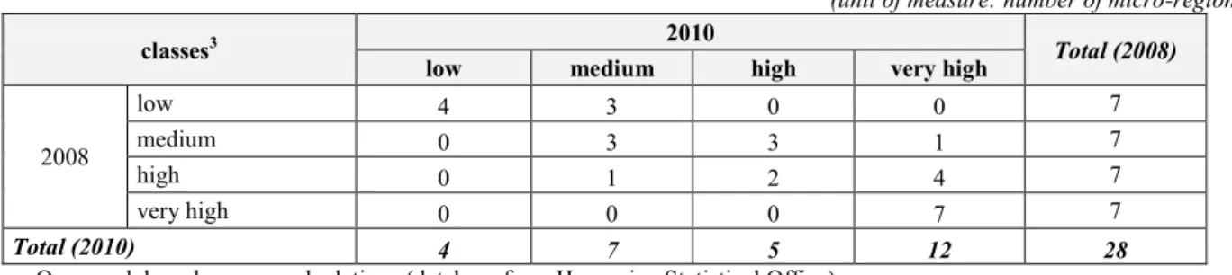
The re-alignments among particular classes are much more significant within Northern Hungary. No change was observable in the case of micro-regions in the very high unemployment group, compared to other groups, from year 2008 to year 2010 (naturally, there were intra-group realignments in each micro-region but the transition matrix does not examine them).
Table 3. One-step transition matrix of North Hungarian micro-regions according to the number of registered job-seekers (from year 2008 to year 2010)
(unit of measure: number of micro-regions)
classes3 2010
Total (2008)
low medium high very high
2008
low 4 3 0 0 7
medium 0 3 3 1 7
high 0 1 2 4 7
very high 0 0 0 7 7
Total (2010) 4 7 5 12 28
Source: Own work based on own calculations (database from Hungarian Statistical Office)
The value of mobility index is 57% in Northern Hungary. The author calculated mobility indices for the rest of the regions as well, trying to find evidence as to whether the realignment among groups was the lowest in Northern Hungary (Table 4).
2 The number of registered job-seekers per thousand person of low unemployment class are: 31-51 people.
The number of registered job-seekers per thousand person of medium unemployment class are: 52-75 people.
The number of registered job-seekers per thousand person of high unemployment class are: 76-100 people.
The number of registered job-seekers per thousand person of very high unemployment class are: 101-143 people.
3 The number of registered job-seekers per thousand person of low unemployment class are: 39-63 people.
The number of registered job-seekers per thousand person of medium unemployment class are: 64-91 people.
The number of registered job-seekers per thousand person of high unemployment class are: 92-111 people.
The number of registered job-seekers per thousand person of very high unemployment class are: 112-158 people.
Table 4. Value of mobility index by regions from years 2008 to 2010
Region Mobility index
Southern Great Plain 61.1%
Southern Transdanubia 55.5%
Northern Great Plain 66.7%
Northern Hungary 57.0%
Central Transdanubia 54.7%
Central Hungary 91.6%
Western Transdanubia 65.8%
Source: Own work based on own calculations (database from Hungarian Statistical Office) Conclusions
In summary, the realignment of micro-regions among classes is of much lower degree within Northern Hungary than in the rest of Hungarian regions, except for Southern Transdanubia and Central Transdanubia. The intra-country realignment was 47.8% from years 2004 to 2008, and it was 53.7% from 2008 to 2010. At the same time, the intra- regional realignment from 2008 to 2010 was of lower degree than in the previous period; that is, a process of inter - regional equalization began in terms of the number of registered job-seekers.
The realignment of the number of registered job-seekers among groups (so called classes) in Northern Hungary was not as significant as in the rest of the regions in Hungary since the economic crisis. The reason for that is that the crisis shook less developed regions to a lesser extent also from labour market perspective. The least realignment in Northern Hungary took place among the least favourable (very high unemployment) and the unfavourable labour market (high unemployment) classes.
This research was realized in the frames of TÁMOP 4.2.4. A/2-11-1-2012-0001. National Excellence Program – Elaborating and operating an inland student and researcher personal support system convergence program. The project was subsidized by the European Union and co-financed by the European Social Fund.
References
1. Bhatnagar S. – Kowshik H.J. (2005): A discrete parameter stochastic approximation algorithm for simulation optimization, Simulation 81, no.11:757-772.
2. Christodoulakis, G. – Mamatzakis, E. C. (2009): Labour market dinamics in EU: a Bayesian Markov Chain Approach, Department of Economics, Discussion Paper Series 2009-07., 1-21.
3. Guha D. – Banerji A. (1999): Testing for regional cycles: a Markov-switching approach, Journal of Economic and Social Measurement 25, 163–
182.
4. Krolzig H.M. – Marcellino M. – Mizon G.E. (2002): A Markov–switching vector equilibrium correction model of the UK labour market, Empirical Economies, no.27: 233-254.
5. Lipták K. (2012): The application of Markov chain model to the description of Hungarian market processes, Zarządzanie Publiczne, nr 4(16)/2011, pp. 133-149.
6. Lu, S.L. 2009. Comparing the reliability of a discrete-time and a continuous-time Markov chain model in determining credit risk, Applied Economics Letters, no.16:1143-1148.
7. Major, K. (2007): Markov láncok használata a regionális jövedelemegyenlőtlenségek előrejelzésében, Tér és Társadalom 21, no.1:53-67.
8. Major, K. (2008): Markov-modellek – Elmélet, becslés és társadalomtudományi alkalmazások, Regionális Tudományi Tanulmányok 14., BCE Markoökonómia Tanszék – ELTE Regionális Tudományi Tanszék 1-189.
9. Toikka R.S. (1976): A Markovian model of labor market decisions by workers, The American Economic Review 66, no.5:821-834.
10. Ugrósdy, Gy. (2002): A világ búza termésének vizsgálata Markov-lánc modell alkalmazásával, Gazdálkodás 46, no.2: 67-71.
Katalin LIPTÁK Ph.D., Dr., assistant lecturer Institute of World and Regional Economics, Faculty of Economics, University of Miskolc, Hungary. Address: Miskolc-Egyetemváros, H-3515, Hungary, E-mail address: liptak.katalin@uni-miskolc.hu. Telephone:
+36-46-565-111/2023 The field of scientific interests: employment policy, regional disparities, labour market situation.