Analysis of Economic Risks in Sow Production
Soltész A1, Szőke Sz2, Balogh P3 A B S T R A C T
We prepared a model farm based on the data of a young pig production farm which has 1300 breeding sows in order to examine the main risk factors affecting the profitability of young pig production. Farrowing and mortality rates, as well as cost and price data were recorded as the input data of the model. Revenue of the farm, total costs, total income and the prime cost of young pig production were used as output. The Monte-Carlo simulation was used in the model for risk assessment.
Based on the results of the analysis, it was concluded that the total income was most affected by the number of piglets per litter (ß=0.691), the total farm costs were most influenced by the indexes related to piglet output (number of piglets per litter:
ß=0.455, price of piglet feed: ß=0.443, feed consumption of piglet: ß=0.364) while the change of the total income of the farm was most determined by young pig price (ß=0.578).
Keywords:
pig production, risk analysis, Monte-Carlo simulation
1. Introduction
Agricultural production is one of the riskiest production activities, since producers have to face numerous risks both in crop production and animal husbandry sectors.
In Hungary, there were significant changes in terms of the distribution of agricultural production between different sectors during the past decade. The role of animal husbandry has been decreasing constantly. Before 2004, its share in the gross output of agricultural production exceeded 40% and it has been fluctuating between only 33-37% since 2004 (KSH, 2013a). However, this decline is mainly the result of the continuous decrease which can be observed in the amount of livestock (in 2012, only the amount of cattle livestock was higher than its 2004 level (KSH, 2013b)). This change has struck the swine livestock the most: the amount of swine livestock was more than 5 million in 2002, while it did not even reach 3 million by the end of 2012 (KSH, 2013c). Further problems of the sector include inefficient production, improper swine keeping technology and foraging technology, while the problems with the economies of scale are also significant problems of the sector. In general, it can be stated that swine progeny is low in Hungary while the increase in body weight is slow, swine reach slaughter age later and the feed conversion efficiency is also weak in Hungary. All these factors create uncertainty for producers, forcing them to end their activity.
It is a well-known fact that the basis of economical swine breeding and pork production is the proper quantity and quality of swine progeny. Consequently, the Hungarian government prepared the so-called “National Swine Strategy” in 2012, with the aim to double the amount of the Hungarian swine livestock. Furthermore, the strategy contains strategic improvement measures in order to work out a breeding, production integration and research and development program (Magyar Közlöny, 2012).
In this study, we aim to examine the conditions of profitable piglet production; i.e., the circumstances under which breeding sows are able to achieve the best production results. Based on the production data of a real breeding farm and the unit prices related to production, we prepared a swine
1 Soltész Angéla
University of Debrecen, 4032 Debrecen, Böszörményi út. 138, Hungary soltesza@agr.unideb.hu
2 Szőke Szilvia
University of Debrecen, 4032 Debrecen, Böszörményi út. 138, Hungary szilvia@agr.unideb.hu
3 Balogh Péter
University of Debrecen, 4032 Debrecen, Böszörményi út. 138, Hungary baloghp@agr.unideb.hu
farm simulation model which helps in preparing predictions of profitability indexes while taking various risk factors into consideration.
2. Risk modelling
The main task of mathematical modelling is to set up the most accurate models of the processes and phenomena going on in the technical system, as well as to evaluate their results. However, when establishing this model, one always has to consider a certain type and amount of uncertainty.
There are several risk factors in animal husbandry mainly due to the uncertainty of yields and market factors. Producers can do little to nothing to prevent these risks. Especially for this reason, it is important to be knowledgeable about how the system works.
Modelling makes it possible to get to know and characterise reality more accurately; therefore, the extent of risk can be quantified, thereby providing information to decision-makers (Pocsai and Balogh, 2011).
Nowadays, due to the development of computers, it is possible to determine and handle risks more easily, faster and also more accurately (Beaver and Parker, 1995). Various complex risk assessment and risk management and simulation strategies are available to users, such as the Monte-Carlo simulation which is a rather widely used numerical procedure. The greatest advantage of the method is that there is no need to set up a model which often uses very complex analytical and numerical methods, but the posed questions can be answered by “only” generating random numbers quickly and efficiently (Kovács and Csipkés, 2010; Takács and Felkai, 2010; Takács-György and Takács, 2011;
Vizvári et al., 2011; Huzsvai et al., 2012).
2.1. Monte-Carlo simulation
Simulation means that the examination of a process or a system is done by using a substitute model whose aim is to make it possible to study the behaviour of the original system. During simulated procedures, the model run and executed temporally (as opposed to the exact results provided by analytical models). The results are representative samples of the performance indexes describing the functioning of the system (Winston, 1997).
One of the alternative methods of risk assessment is the Monte-Carlo simulation, during which the modelling of the system is followed by computerized simulations which use random values in accordance with the system. The way the system works is that values are chosen randomly based on the probability distributions attributed to each uncertain factor. These values are then used in each experiment of the simulation analysis (Russel and Taylor, 1998; Vose, 2006).
As the first step of the simulation, the influential (input) variables, their possible range, probability distribution and the correlation between each variable are recorded in the model to be analyzed. The values of the variables in the given interval and distribution are generated by a random number generator (Szőke et al., 2010). Furthermore, result (output) variables are also recorded. Finally, the model is run several consecutive times on a computer, usually with experiment numbers of 1000- 10000. As a result of simulation, an expected value and standard deviation range is obtained for each response variable. Furthermore, the distribution function will make it possible to determine the probability of whether the value of the given variable will fall within the given range (Winston, 2006).
By increasing the number of model runs, the distribution of the response variable can be set with optional accuracy in accordance with the following (Watson, 1981; Jorgensen, 2000):
(1)
ψ
=Eπ{U(X)}=∫
U(x)π
(x)dxwhere X = {θ, ø} is a vector with θ decision parameters and ø condition parameters, π is the distribution of x and U(x) is a utility function which usually refers to income. Based on these, the Eπ () function provides the expected utility with given distribution.
The running and practical implementation of the simulation is done with a simulation software, several of which is based on the well known spreadsheet application Excel. An example is @Risk
(Palisade Corporation). We used version 4.5 of this software to perform the simulation analysis of our swine farm model (Palisade, 2005).
2.2. Description of the farm which served as a basis of the model
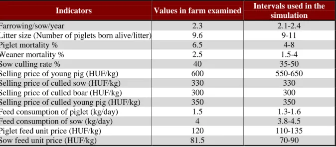
Our model was set up based on the 2013 data of a breeding farm located in the Northeastern region of Hungary. The farm has 1300 sows and it produces more than 26 000 young pigs a year. The young pigs are sold at the age of 90 days when their body weight is 36 kg. The main production indexes of the farm are shown in Table 1. The intervals used in the simulation were determined by the aid of the experts.
Table 1. Values of the farm indicators and market factors and intervals used in the simulation Indicators Values in farm examined Intervals used in the
simulation
Farrowing/sow/year 2.3 2.1-2.4
Litter size (Number of piglets born alive/litter) 9.6 9-11
Piglet mortality % 6.5 4-8
Weaner mortality % 2.5 1.5-4
Sow culling rate % 40 35-50
Selling price of young pig (HUF/kg) 600 550-650
Selling price of culled sow (HUF/kg) 330 330
Selling price of culled boar (HUF/kg) 300 300
Selling price of culled young pig (HUF/kg) 350 350
Feed consumption of piglet (kg/day) 1.5 1.3-1.6
Feed consumption of sow (kg/day) 4 3.8-4.5
Piglet feed unit price (HUF/kg) 120 110-135
Sow feed unit price (HUF/kg) 81.5 70-90
2.3. Structure of the model
Using the indexes of the farm, we used Excel to prepare our model for production and profitability of the breeding farm. This was followed by providing the variables to be used in the simulations, as well as their potential ranges and probability distributions which were set using @Risk 4.5 running in the spreadsheet application. The following input parameters were involved in the model as influential factors:
• Farrowing/sow/year (FSY)
• Litter size (LS)
• Piglet mortality (PM)
• Weaner mortality (WM)
• Sow culling rate (SCR)
• Selling price of young pig (PYP)
• Feed consumption of piglet (FCP)
• Feed consumption of sow (FCS)
• Piglet feed unit price (PFP)
• Sow feed unit price (SFP)
The assumed distribution of the parameters can be chosen from several distribution types of which we decided to use the triangular distribution. This type of distribution is a continuous probability distribution with lower limit a, upper limit b and mode c, where a < b and a ≤ c ≤ b. The probability density function is given by
(2)
<
≤
− <
−
−
≤
− ≤
−
− <
=
, 0
) )(
(
) ( 2
) , )(
(
) ( 2
, 0
) , , (
x b for
b x c c for
b a b
x b
c x a a for
c a b
a x
a x for
c b a x f
whose cases avoid division by zero if c = a or c = b (Evans et al., 2000). This distribution is generally used if both the minimum, maximum and most probable values are known. The ranges used by us are shown in Table 1 and the most probable values were considered to be the mean farm values.
Of the input data, we set a correlation value of 0.9 between the piglet and sow feed unit prices, thereby showing the strong positive correlation between feed prices.
Five farm indexes were provided as output variables of the simulation:
• Total farm revenue (HUF)
• Total farm costs (HUF)
• Total farm income (HUF)
• Prime cost (HUF/young pig)
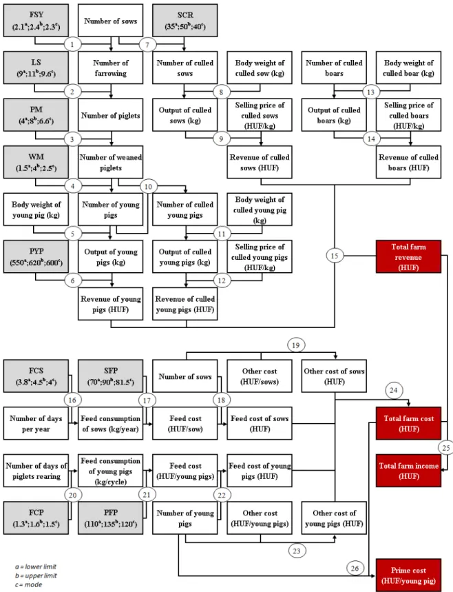
After setting the above parameters, the simulation model (Figure 1) was run with 10 000 replications and sensitivity analyses were performed on the output variables.
The sensitivity analysis was carried out based on standardized coefficients of regression (ß) and Spearmann’s rank correlation coefficients. The former is an index expressing the impact of the explanatory (input) variable which is obtained if both the dependent and the explanatory variables are used in a standardized form and not in their original measurement units (Moksony, 2006). The significance of this index is that it shows the rank of importance of the explanatory variables independently of their measurement units (Hajdú, 2003). Also, this index made it possible to rank the input variables from the aspect of risk. The sign of the coefficient also gives information about the direction of change (Szőke et al., 2010). If the sign is positive, an increase of the input results in an increase of the output variable. However, if the sign is negative, an increase of the input causes the decrease of the output.
Figure 1. Description of the simulation model Equations in the simulation model:
1: Number of sows x Farrowing/sow/year (FSY) 2: Number of farrowing x Litter size (LS)
3: Number of piglets x [1 - Piglet mortality % (PM)]
4: Number of weaned piglets x [1 - Weaner mortality % (WM)]
5: Number of young pigs x Body weight of young pig (kg)
6: Output of young pigs (kg) x Selling price of young pig (HUF/kg) (PYP) 7: Number of sows x [1- Sow culling rate % (SCR)]
8: Number of culled sows x Body weight of culled sow (kg)
9: Output of culled sows (kg) x Selling price of culled sow (HUF/kg) 10: Number of weaned piglets - Number of young pigs
11: Number of culled young pigs x Body weight of culled young pig (kg)
12: Output of culled young pigs (kg) x Selling price of culled young pig (HUF/kg) 13: Number of culled boars x Body weight of culled boar (kg)
14: Output of culled boars (kg) x Selling price of culled boar (HUF/kg)
15: Revenue of culled sows (HUF) + Revenue of culled boars (HUF) + Revenue of young pigs (HUF) + Revenue of culled young pigs (HUF)
16: Feed consumption of sow (kg/day) (FCS) x Number of days per year 17: Feed consumption of sow (kg/year) x Sow feed unit price (HUF/kg) (SFP) 18: Feed cost (HUF/sow) x Number of sows
19: Other cost (HUF/sow) x Number of sows
20: Feed consumption of piglet (kg/day) (FCP) x Number of days of piglets rearing 21: Feed consumption of pig (kg/cycle) x Piglet feed unit price (HUF/kg) (PFP) 22: Feed cost (HUF/young pig) x Number of young pigs
23: Other cost (HUF/young pig) x Number of young pigs
24: Feed cost of sows (HUF) + Other cost of sows (HUF) + Feed cost of young pigs (HUF) + Other cost of young pigs (HUF)
25: Total farm revenue (HUF) - Total farm cost (HUF) 26: Total farm cost (HUF) / Number of young pigs 3. Results
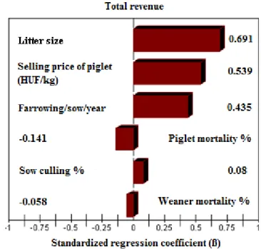
During the performed modelling, the first step was to examine the factors affecting the amount of total farm revenue. Based on the tornado diagram of the sensitivity analysis (Figure 2), it can be concluded that the average litter size affects the total revenue the most. The change of standard deviation of the number of piglets per litter by 1 results in a 0.691 (ß) change of the standard deviation of the total revenue. Furthermore, the change of piglet price (ß=0.539) and the number of farrowing per sow per year (ß=0.435) also has a significant impact on the total revenue. All three indexes are in a moderately close correlation with revenue, (Spearmann’s rank correlation coefficient: 0.43 - 0.69), showing that the increase of these indexes will result in the increase of revenue.
Figure 2. Tornado chart of the standardized regression coefficient pertaining to the total revenue
Mortality/culling rates also affect revenue. The ß coefficient with the highest absolute value was obtained in the case of piglet mortality, meaning that the change of the standard deviation of mortality by 1 results in a 0.141 change in the standard deviation of revenue in the opposite direction, since the negative sign refers to the fact that the decrease of the mortality rate results in the increase of revenue.
As regards the other indexes, the value of the standardized coefficient of regression was nearly zero (|ß|<0.1).
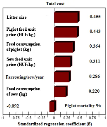
Figure 3. Tornado chart of the standardized regression coefficient pertaining to the total cost The next examined output was the total farm costs (Figure 3), the value of which was affected by the number of piglets per litter (as farm index) and piglet feed price (as market index) the most. In both cases, it can be stated that the change of standard deviation by 1 results in a change of more than 0.4 in the standard deviation of the total farm costs.
The feed consumption of piglets, the sow feed price, the farrowing/sow/year ratio and the feed consumption of sows also play an important role (ß=0.22-0.44) in shaping farm costs; therefore, the increase of these values also result in the increase of total costs.
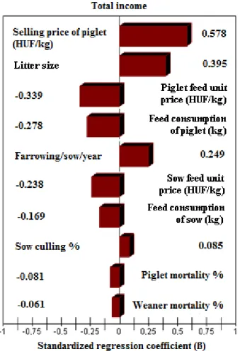
The result of the sensitivity analysis of the income calculated from the difference between the farm revenue and total costs is shown in Figure 4. Based on the obtained values, it can be established that income is most affected by the change of piglet price of the variables, greatly determining the amount of revenue (Spearmann’s rank correlation: 0.57). The change of the standard deviation of piglet price by 1 results in a 0.578 change in the standard deviation of total income. The increase of the number of piglets also causes the income to increase (ß=0.395), but to a lower extent than in the case of revenue, since the higher amount of piglets also results in increasing expenses.
Figure 4. Tornado chart of the standardized regression coefficient pertaining to the total income The input factors which positively affected the total costs are shown in the figure of income with the same rank, but with an opposite sign. The absolute value of the standardized coefficient of regression was around 0.3 in the case of the factors affecting the feeding of piglets. Factors affecting the feeding of sows caused a somewhat smaller change (|ß|=0.2).
The standardized coefficient of regression and the Spearmann’s rank correlation coefficient were close to zero (|ß|<0.1) in the case of all other input variables.
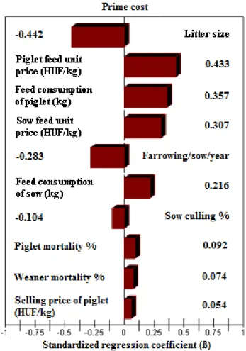
Since the main profile of the farm is young pig production, we considered it to be important to examine also the factors affecting the prime cost of young pig. Figure 5 shows the tornado diagram of the sensitivity analysis of the specific prime cost of young pig production.
Figure 5. Tornado chart of the standardized regression coefficient pertaining to the piglet prime cost It can be seen in the figure that the highest value of the standardised coefficient of regression was obtained in the case of the number of piglets per litter (|ß|=0.442), but it has a negative sign. This value can be interpreted in a way that the increase of the standard deviation of the litter size by 1 results in a 0.442 decrease in the standard deviation of the prime cost of young pig production. Changes in the unit price of feed and feed consumption also show significant influence (the rank of significance of each variable and the values of the standardised coefficient of regression are the same as in the case of total costs). As opposed to the negative value of the number of piglets, these indexes have positive ß values, i.e., the increase of the index results in increasing specific prime cost. Furthermore, the impact of the change in case of the number of litters per sow is also worth mentioning. The increase of the standard deviation of this index by 1 results in a 0.283 decrease in the standard deviation of the prime cost.
The main descriptive statistic of the response variables employed in the simulation analysis are summarized in Table 2.
Table 2. Descriptive statistic simulation outputs
Outputs Min Mean Max Std. Dev. Skewness Kurtosis Total revenue (million HUF) 511,6 612,5 753,1 35,9 0,29 2,87
Total cost (million HUF) 498,6 575,5 687,5 25,6 0,19 2,84
Total income (million HUF) -70,2 37,1 158,2 33,4 0,09 2,85 Prime cost (HUF/young pig) 17 519 20 361 23 438 921,7 0,06 2,78
The widest range can be observed in the case of the total income with a relative standard deviation value of 90%. This means that the value of the simulated mean does not properly characterize the expected income.
Figure 6. Relative frequencies of the prime cost (HUF/young pig) after 10.000 simulation runs Figure 6 shows the prime cost histogram of one young pig after performing the 10 000-simulation experiment. The mean value was 20 361 HUF per young pig which equals 565.68 HUF per kg prime cost if it is related to 36 kg body weight. The interquartile range is between 19714 - 20989 HUF per piglet which equals 548-583 HUF per kg.
4. Conclusion
The consideration and measurement of risk elements help in making a more informed decision. In this study, we performed the analysis of the occurring risks of sow breeding using simulation modelling. The main production and economic parameters were incorporated into the model as stochastic variables. After the Monte-Carlo simulation was run, we examined how each risk factor affects the farm revenue, risk and income, as well as the specific prime cost of piglets.
Based on our results, it can be stated that the litter size was the most influential factor of the natural farm indexes. The number of piglets per litter had the following ß values, representing its influence on the following factors: the variability of total revenue: 0.691; variability of total costs: 0.455; variability of total income: 0.395; variability of the specific prime cost of young pig production: -0.442.
Consequently, the management of the farm is recommended to pay more attention to satisfying the needs of the sows at the farm in order to reach the highest possible progeny in the case of each breeding sow.
Of the influential market factors, the selling price of young pig had the highest impact on the variability of total revenue (ß=0.539) and total income (ß=0.578). Furthermore, the impact of piglet feed price is worth mentioning, showing an influence of ß=0.443 on the standard deviation of total costs and ß=0.433 on the standard deviation of the prime cost of young pig production. The safety of production is necessary to be increased both from the aspect of acquisition and sales by means of minimizing the change of input and output prices. This could be facilitated by arranging collective acquisition and sales with other producers.
Of the data modelled by us, the mortality/culling rates had the lowest significance, as the coefficient of correlation of the tornado diagrams was nearly zero (|r|≤0.1).
Acknowledgements
Angela Soltesz’s research was realized in the frames of TÁMOP 4.2.4. A/2-11-1-2012-0001
„National Excellence Program – Elaborating and operating an inland student and researcher personal support system convergence program”. The project was subsidized by the European Union and co- financed by the European Social Fund.
This paper was supported by the János Bolyai Research Scholarship of the Hungarian Academy of Sciences, in additional it was subsidized by the Research Scholarship of the University of Debrecen.
References
Beaver, W.H., Parker, G. 1995. Risk Management: Problems and Solutions. Stanford University.
Evans, M., Hastings, N., Peacock, B. 2000. Triangular Distribution, In Statistical Distributions, 3rd ed. New York, pp. 187-188.
Hajdú, O. 2003. Többváltozós statisztikai számítások. Központi Statisztikai Hivatal, pp. 215.
Huzsvai, L., Megyes, A., Rátonyi, T., Bakó, K., Ferencsik, S. 2012. Modelling the soil-plant water cycle in maize production: A case study for simulation of different soving dates on chernozem soil. Növénytermelés 61.
pp. 279-282.
Jorgensen, E. 2000. Monte Carlo simulation models: Sampling from the joint distribution of “State of Nature”- parameters. In: Van der Fels-Klerx, I.; Mourits, M. (eds). Proceedings of the Symposium on “Economic modelling of Animal Health and Farm Management”, Farm Management Group, Dept. of Social Sciences, Wageningen University, pp. 73-84.
Kovács, S., Csipkés, M. 2010. A case study of crop structure modelling and decision making by using a stochastic programming model. Agrárinformatika Folyóirat, 1(1) pp. 1-7.
http://journal.magisz.org/files/journals/JAI_Vol_1_No_1.pdf Központi Statisztikai Hivatal 2013a. Mezőgazdaság, 2012.
http://www.ksh.hu/docs/hun/xftp/idoszaki/mezo/mezo12.pdf
Központi Statisztikai Hivatal 2013b. Állatállomány, 2012. December 1., Statisztikai tükör VII. Évf. 12. szám http://www.ksh.hu/docs/hun/xftp/idoszaki/allat/allat1212.pdf
Központi Statisztikai Hivatal 2013c Gyorstájékoztató http://www.ksh.hu/docs/hun/xftp/gyor/all/all21306.pdf
Magyar Közlöny 2012. A Kormány 1323/2012. (VIII. 30.) Korm. Határozata a sertéságazat helyzetét javító stratégiai intézkedésekrõl, 2012. évi 114. szám, 19447-19449. p.
http://www.kormany.hu/download/7/76/a0000/KH_2012_1323_%28VIII_30%29_Kormanyhatarozat.pdf Moksony, F. 2006. Gondolatok és adatok. Társadalomtudományi elméletek empirikus ellenőrzése, Aula Kiadó, Budapest, pp. 205.
Palisade 2005. @RISK advanced risk analysis for spreadsheets, Version 4.5. Palisade Corporation 22, pp. 116.
Pocsai, K., Balogh, P. 2011. A @RISK program bemutatása egy sertéstelepi beruházás esettanulmányán keresztül, Agrárinformatika Folyóirat, 2(1) pp. 77-85.
http://journal.magisz.org/files/journals/JAI_Vol_2_No_1.pdf
Russel, R.S., Taylor, B.W. 1998. Operations Management, Focusing on quality and competitiveness, New Jersey.
Szőke, Sz., Nagy, L., Balogh, P. 2010. Monte-Carlo szimuláció alkalmazása a sertéstelepi technológia kockázatelemzésében, Acta Agraria Kaposváriensis, 14(3) pp. 183-194.
Takács, I., Felkai, B.O. 2010. Simulation model for estimating risk of uncertainty on return on investments of public investments, Delhi Business Review 11(1) pp. 29-42.
Takács-György, K., Takács, I. 2011. Risk Assessment and Examination of Economic Aspects of Precision Weed Management, Sustainability 3, pp. 1114-1135.
Vizvári, B., Lakner, Z., Csizmadia, Z., Kovács, G. 2011. A stochastic programming and simulation based analysis of the structure of production on the arable land, Annals of Operations Research 190(1) pp. 325-337.
Vose, D. 2006. Risk analysis, John Wiley&Sons Ltd., New York.
Watson, H. 1981. Computer Simulation in Business, Whiley, New York
Winston, W.L. 1997. Operations Research Applications and Algorithms, Wadswoth Publishing Company.
Winston, W.L. 2006. Financial modells using simulation and optimization, Palisade Corporation, Newfield. pp.
505.