Estimation of dissolved oxygen in riverine ecosystems: Comparison of differently optimized neural networks
Abstract
Dissolved oxygen is one of the most important water quality parameters in relation to aquatic life, and one of the most direct indicators of water pollution. The present study employs a novel methodology for the estimation of riverine dissolved oxygen using neural network models taking the spatial homogeneity of the water quality sampling sites into account. In three alternative configurations, a multivariate linear regression model, a radial basis function neural network and a general regression neural network are applied to discover which is best able to forecast dissolved oxygen effectively. Data from 13 water quality monitoring stations of the River Tisza are used, including runoff, water temperature, electric conductivity and pH. The three configurations are as follows: (i) a randomly chosen training and test set (which is then considered the reference model), (ii) a training and test set chosen in a spatially controlled way and (iii) a data set composed of two homogeneously behaving sampling sites with the addition of the site lying closest to these downstream. It was found that if the input of the linear model or the neural networks consists of a group or groups of sampling sites displaying homogeneous behavior, better performance is achieved in the estimation. Specifically, the best estimation of dissolved oxygen was achieved in the middle and lower reaches of the river, with an average of 81% and 87% of variance explained, respectively; the General Regression Neural Networks gave the best performance, in the middle reaches: 85%, and 90% in the lower ones, respectively, even in the presence of a high degree of anthropogenic activity, as is the case with the River Tisza.
Keywords: Combined cluster and discriminant analysis; Dissolved oxygen forecasting; General regression neural networks; Radial basis function neural network; Homogeneous sampling sites
1
Introduction
The presence of a sufficient amount of dissolved oxygen (DO) in water is essential for the higher forms of aquatic life to flourish ( Connolly et al., 2004; Dodds, 2002 ). The issues associated with low concentrations of DO in rivers have been recognized for about a century ( Thompson, 1925 ). Low DO content can cause an adverse change in the composition of riverine assemblages ( Connolly et al., 2004 ), as well as fish mortality, odors and other aesthetic nuisances ( Cox, 2003 ).
Regular DO dynamics are complex, involving interactions between physical, chemical, and biological processes ( Wang et al., 2003 ). Oxygen can enter the water via two main routes: by direct absorption from the atmosphere, and as a by-product of photosynthesis ( Odum, 1956; Schurr and Ruchti, 1977 ). The amount of DO in an aquatic environment is determined by the various turns in the continuous balancing act between oxygen-producing and oxygen-consuming processes ( Heddam, 2014 ). Natural waters in equilibrium with the atmosphere typically contain DO concentrations in the range of 5 to 15 mg L-1 O2 depending on water temperature, salinity, and altitude ( APHA, 1998 ). The analysis of this DO content is extremely important in the determination of water quality. Besides its direct measurement, its values are commonly estimated using various deterministic hydrological models (e.g. Soil and Water Assessment Tool, Water Quality Analysis Simulation Program, QUAlity Simulation Along Rivers, Better Assessment Science Integrating Point and Non-point Sources (see Wang et al., 2013 )) and statistical models (e.g. Autoregressive integrated moving average model (ARIMA), Analysis of variance). It should be pointed out, however, that these hydrological models are very complex and their application requires a large amount of input information and computational capacity ( Kanda et al., 2016; Najah et al., 2011 ), neither of which may necessarily be available in a given instance ( Šiljić Tomić et al., 2016 ).
Anita Csábrágia csabragi.anita@gmail.com, Sándor Molnára molnar.sandor@gek.szie.hu, Péter Tanosa tanospeter@gmail.com, József Kovácsb kevesolt@geology.elte.hu, Márk Molnárc molnar.mark@gtk.szie.hu, István Szabóa Szabo.Istvan@gek.szie.hu, István Gábor Hatvanid,⁎ hatvaniiig@gmail.com
aDepartment of Informatics, Szent István University, Páter K. u.1., Gödöllő H-2103, Hungary
bDepartment of Physical and Applied Geology, Eötvös Loránd University, Pázmány Péter sétány 1/C., Budapest H-1117, Hungary
cDepartment of Macroeconomics, Szent István University, Páter K. u.1., Gödöllő H-2103, Hungary
dInstitute for Geological and Geochemical Research, Research Centre for Astronomy and Earth Sciences, MTA Budaörsi út 45, Budapest H-1112, Hungary
⁎Corresponding author at: Institute for Geological and Geochemical Research, Research Center for Astronomy and Earth Sciences, MTA, Budaörsi út 45., Budapest H-1112, Hungary.
i The corrections made in this section will be reviewed and approved by journal production editor.
Track-changes version of proof of Csábreági et al., 2019. Ecological Engineering, 138, 298-309
In the case of rivers, DO dynamics may be taken as being in a linear relationship with water temperature, if it is the only driving factor considered. However, in most cases due to the nature of the flow system, and the presence of turbidity, anthropogenic effects, wastewater channeling, etc. the behavior of DO should rather be considered as nonlinear, as it depends on the combination of multiple environmental factors (Chen and Liu, 2014). It should be noted that there are few methodological approaches onat hand to tackle this obstacle. In such circumstances, Artificial Neural Networks (ANNs) may provide a solution. Their use necessitates more sophisticated regression models based on, for instance, Machine Learning (Shaikhina and Khovanova, 2017), which can be utilized by ANNs.
Artificial neural networks are flexible modeling tools and are able to approximate accurately complicated non-linear input–output relationships (Palani et al., 2008). This approach has gained widespread acceptance as a potentially useful way of modeling hydrological processes, having been applied to a range of different problems, including water quality, rainfall runoff, sedimentation and rainfall forecasting (Emamgholizadeh et al., 2014, Várbíró et al., 2007).
When neural networks are employed, the data set is broken down into at least two subsets: the training and test sets, and the performance of the various models is influenced fundamentally by the definition of these sets. Three alternatives exist for the division of the sample set into these subsets.
In most cases, an arbitrary division is made when defining the training and test sets. In such cases, the given output is simulated and modeled for the complete system, ignoring the possibility of input optimization (for dissolved oxygenDO estimation with ANNs in rivers e.g. Antanasijević et al., 2014; Basant et al., 2010; Emamgholizadeh et al., 2014; Heddam, 2014; Kanda et al., 2016; Wen et al., 2013). This division can also be made done in a non-arbitrary way. For example, the: nine sampling points inof the Harsit stream in Turkey were divided in such a manner that all the structures of the data set were included in both the training and test sets (Bayram and Kankal, 2015, Table A1).
In the literature, there is a smaller number of cases in which the total dataset is divided temporally into several time intervals. The larger dataset is then used as the training set, and the smaller, with the later usually consisting of data from the ultimate period(s)data, for testing. This procedure may be considered a kind of temporal forecasting (see for example: Antanasijević et al., 2013; Ay and Kisi, 2012; Csábrági et al., 2017, 2015; He et al., 2011; Singh et al., 2009; Šiljić Tomić et al., 2016, 2018b).
In an even smaller number of cases, the total dataset is divided into training and test sets according to the sampling locations. For example, on the Melen River, Turkey, of the total of eight sampling points, four were used for training and four for testing (Dogan et al., 2009). Since the assigned sampling points in the sets were not adjacent, but rather sporadically distributed and randomly chosen for incorporation into the model, this procedure cannot be regarded as spatial forecasting, only as modeling or simulation.
One example of temporal forecasting was found, in this case coupled with spatial modeling; this had been undertaken at two sampling locations (upstream, downstream) on the Arkansas River in Colorado (Ay and Kisi, 2012). In every case, the accuracy of the estimation of an ANN model is fundamentally determined by the input, that is, by the structure of the sample set. Multiple sources deal with the optimization of the ANN’s sample set, which can be approached from many angles.
The optimization of ANNs can be approached from many angles:
(i) by choosing the most appropriate set of input parameters to maximize the explained variance with the lowest number of parameters (by using e.g.
correlation matrices, variance inflation factor, smoothing factors of the individual parameters) (Antanasijević et al., 2014; Ouyang, 2018; Prasad et al., 2017),
(ii) by choosing a set of samples in space which account for most of the variance in the full dataset
(iii) by choosing such time intervals as will again account for most of the variance and in which the data are more homogenous (e.g. by cluster analysis or applying ANNs);
Numerous sStudies which show examples for all three optimizations may be found in literature, (e.g. Šiljić Tomić et al., 2016, 2018b .)
The objective of thise present study is to demonstrate the applicability of a novel methodology for estimating dissolved oxygen at water quality sampling sites on the second largest river in Central Europe. In the present instance, this was done by taking into account the spatial homogeneity of groups of sampling sites along a river section to which artificial neural networks were then applied. A key question was whether it is possible to improve spatial forecasting by choosing training and test sets in a directed and conscious manner and by taking into consideration the spatial homogeneity of the river.
2
Materials and methods
2.1 Study area
The River Tisza (Fig. 1) is the largest tributary of the River Danube, and the second largest river in Hungary. It collects the waters of the northern part of the Carpathian Basin, and as such, it is also an important ecological corridor. It rises in the Ukraine and flows into the Danube at Titel, in the Vojvodina, Serbia. Its watershed is 157,186 km2, and of this, approximately one-third lies in Hungary (47,000 km2). Its total length is 966 river km (rkm), across five countries (the Ukraine, Romania, Hungary, Slovakia and Serbia). Its Hungarian tributaries in downstream order of their confluences are: the Szamos, Bodrog, Sajó, Zagyva, Kőrös and Maros.
Not only the tributaries and other inflows, but also artificial installations have a major impact on water quality, e.g. dams/water barrage systems ( Kentel and Alp, 2013; Moreira and Poole, 1993 ); of particular significance is the Tiszalök water barrage system at Tiszalök and its reservoir, the Kisköre Reservoir (a.k.a. Lake Tisza), an artificial lake created in 1973 as part of the hydroelectric power plant, and which became the second largest in Hungary. Nowadays, a popular tourist destination and natural reserve, its length is 27 km, average depth 1.3 m, and total area 127 km2.
In this particular setting, it has been observed that in the headwater of the hydropower plant planctic algae are more abundant than upstream in the free-flowing river. This is due to the increased residence time (lower flow velocity) of the water, resulting in lower turbidity and much higher transparency (Tanos et al., 2011 ). Therefore, the dam-tailwater will have low dissolved oxygen, not because of the dam itself, but because of the ecological dynamics of the reservoir upstream of the dam (Bevelhimer and Coutant, 2006). This is generally the case in the absence of sustained photosynthetic oxygen production, because the waste- assimilating capacities of headwater ponds are often much lower than those of free-flowing upstream reaches (Butts and Evans, 1978). Efforts have been made to increase dam-tailwater DO release by e.g. turbine venting; ( for further examples see ERPI, 2002).
Nonetheless, if the water is nutrient rich but not grossly polluted, excessive algal growth can be expected in the headwater, resulting in supersaturated DO levels (ISWS, 1978; Ruane and Hauser, 1991)
Besides these localized point-sources (e.g. treated sewage outflows, tributaries) the diffuse fertilizer input from the agricultural land, along with the environmental impact of the larger urbanized areas of Szeged and Szolnok also significantly impairs water quality (Kovács et al., 2017; Tanos, 2017).
Bi-weekly measured water quality data was available for the years 1998–2003 from 13 sampling locations along the Tisza (Fig. 1).
Replacement Image: Fig1_rev.png
Replacement Instruction: Please replace Fig. 1 with the attached file. Thank you!
2.2 Water quality data set
The appropriate selection of input parameters is a decisive step in the process of estimation. For the estimation of dissolved oxygen content (DO), the bi-weekly data of four water quality parameters were used, measured at 13 sampling locations bi-weekly from 1998 to 2003 ( Figure 1 [Instruction: Please abbreviate Figure to Fig.
]). The parameter selected as most important was runoff (Q, m3 sec-1), which is fundamental for large rivers ( Kovács et al., 2015; Tanos et al., 2015), and which is frequently used in ANN analyses when estimating DO content ( Antanasijević et al., 2013; Ay and Kisi, 2012 ). Temperature (Tw, °C) is widely considered one of the most important parameters in DO content estimation (see, e.g. Bayram and Kankal, 2015; Šiljić Tomić et al., 2018a; Wen et al., 2013 ). Two further parameters were considered as relevant to DO estimation, pH and electric conductivity (EC; μS cm−1). The former was included because its change in a negative direction may reflect communal sewage input ( Verma and Singh, 2013 ) and/or the increased decomposition of organic matter ( Akkoyunlu et al. 2011 ); this, in turn, decreases the DO content. Moreover, from a methodological point of view pH is frequently used in the estimation of the DO content of lake- and river waters (for details see for example: Bayram and Kankal, 2015; Csábrági et al., 2017; Šiljić Tomić et al., 2018a ). On the other hand, conductivity (μS cm−1) was chosen since it is a direct indicator of the ion content (dissolved salts) of water ( Heddam, 2014; Kanda et al., 2016 ).
It should also be noted that the set of parameters chosen for the study is one comprising those frequently used for estimating DO content in rivers, as they are quickly and easily measured ( Bayram et al., 2015 ), thus only a very few data are missing from their time series.
2.3 Steps of analysis and used terminology
In terms of how the training and test data were chosen in the study, three configurations are presented, all in the proportions of 2:1, the training to test data.
In the first configuration (Tisza configuration 1, TC1 for short, Table A2 ), the whole dataset (i.e. all sampling locations) pertaining to the River Tisza was considered and subsequently divided in a random way into the training and the test sets. In this case, DO content is modeled over the entire Hungarian section of the river (594.5 rkm). Technically, the random selection of the data was conducted using three different setups, three separate, randomly chosen, but documented seed values. These will be referred to in the study as TC1-A, TC1-B and TC1-C, where the final letters indicate the different setups. Most frequently, the models with the randomly selected data are the reference ones in NN studies, thus in the present case this first configuration was chosen to serve as the reference for the other two configurations.
Fig. 1
Figure Replacement Requested
Sampling sites on the Hungarian section of the River Tisza A) and the pairwise differences between neighboring sampling locations calculated using CCDA B). Circles of the same color (A) and the negative values (B) indicate that the given sites form a homogeneous group of sampling sites. LDA in panel (B) stands for linear discriminant analysis.
In the second configuration (TC2, Table A2), once again the whole dataset was considered, and four setups were created. In each setup, four neighboring locations were selected as the test set, and the remaining nine locations were used for training. In this way, the desired approx. 2:1 proportion was maintained. In the first setup (TC2-A), the first four sampling sites were considered (T01-T04), then from T04 to T07 (TC2-B), T07-T10 (TC2-C) and finally T10-T13 (TC2- D). With the use of this configuration, "spatial forecasting" was attained for DO, as the training and test sets were selected in a controlled manner.
Finally, in the third configuration (TC3, Table A2), the spatial homogeneity of the data was taken into account as an additional factor. Specifically, the previously obtained homogeneous grouping of sampling sites (Tanos et al., 2015) identified using combined cluster and discriminant analysis (CCDA; Kovács et al., 2014) was utilized, and in this configuration, only three subsets of the whole river were considered. It had been previously documented that the 13 sampling locations of the River Tisza can be assigned to 10 homogenous groups (Tanos et al., 2015; Fig. 1). Three of the groups contain two sampling locations, one each in the upper- middle- and lower reaches (Fig. 1B). CCDA was then employed to group samples or, in the present case, sampling locations; this grouping involved not simply assigning them to similar/optimal groups or subsets, but homogeneous ones (Kovács et al., 2014, 2015). [Instruction: please add an enter here, so "In realtion to this,..." would start in a new paragraph. Thank you!
]In relation to this, the key point of CCDA is that it compares all combinations of hierarchical cluster groups to random groupings and suggests the further division of the obtained cluster groups using a difference value obtained from linear discriminant analysis (Kovács et al., 2014). If this difference value is negative, the grouping obtained is homogeneous, and if not, then further division is required (Kovács et al., 2014).
Since the size of the homogeneous groups of sampling sites was a maximum of two sites in the multisite groups, a third location had to be considered, aside from the two composing the homogeneous groups, in the ANN runs. In the present instance, this was always the neighboring downstream sampling location. In the first setup of Configuration 3, the first homogeneous group of sampling sites and the neighboring downstream site were considered (TC3-A), then the second homogeneous group, plus one site (TC3-B), followed by the third (TC3-C); in all setups, nine sub-setups were examined, on the basis of two sites providing the training, and one the test data. Therefore, in the third configuration, nine sub-setups were investigated, ranging from TC3-A#1 to TC3-C#3.
In the different setups, two kinds of neural networks were employed for estimation: Radial Basis Function Neural Networks (RBFNN; see the details in ), and General Regression Neural Networks (GRNN; see in SOM). Additionally, a multivariate linear regression (MLR, Draper and Smith, 1981, Reddy, 2011) model was used. This latter was used as a reference to compare the performance of the different ANNs with (Ji et al., 2017), as in numerous other studies (e.g. Antanasijević et al., 2013; Ay and Kisi, 2012; Bayram and Kankal, 2015; Heddam, 2014; Ji et al., 2017); the aim was to ensure the replicability of the applied methodology.
Data were preprocessed: (i) as the necessary first step in any modeling procedure outlying and extreme values (Fig. A2) were removed from all the used datasets (Ben-Gal, 2010) following a robust univariate approach introduced by Mosteller & Tukey (1977). The boxplot approach is based on the distribution quadrants ( Ben-Gal, 2010), and is frequently used in ANN studies, such as the one estimating dissolved oxygen in the Danube (Šiljić Tomić et al., 2018a), and (ii) values were standardized before their use as ANN input. Model performance was characterized by metrics: root mean square error (RMSE) and the Pearson coefficient of determination (R2) (Legates and McCabe, 1999).
To give a little more detail, the different setups/sub-setups, methodological approaches and an additional geographical factor were considered and compared to obtain an overview of which section of the river and which model and data structure would provide the most reliable estimation.
The neural networks were implemented in MATLAB (Neural Network Toolbox, Demuth and Beale, 2000), MS- Excel Data Analysis ToolPak was used for MLR analyses, the contour maps were drawn using Golden Software SURFERurfer, and CCDA (Kovács et al., 2014) was applied using R 3.5.0 (R Core Team, 2018).
3
Results
3.1 Overview of the data
The descriptive statistics of the 13 sampling locations on the River Tisza were examined for the years 1998 to 2003 to obtain an overall picture of the water quality characteristics of the various river sections (Table 1, Fig. A2). It was observed that the average runoff of the river quadruples from Tiszabecs (entry point of the river into the country) to Tiszasziget (the last sampling site in Hungary), while it has also been observed that the flow velocity decreases parallel to this ( Hatvani et al., 2018; EC, 2015). Heading downstream, the pH of the river can be considered quasi constant, while EC increased by 50% (Table 1).
Supplementary Online Material (SOM)
Table 1
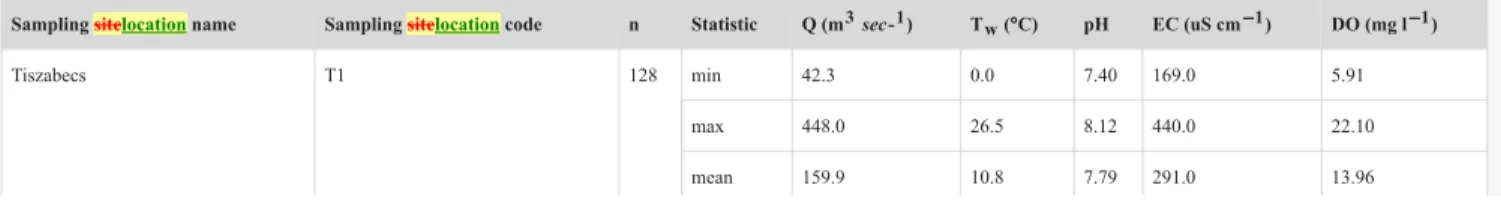
Descriptive statistics of the 13 sampling locations on the River Tisza after data filtering (CV: coefficient of variation; n: number of samples). US-WBS and DS-WBS stand for the sampling sites upstream and downstream of the Tiszalök water barrage system, respectively.
Sampling sitelocation name Sampling sitelocation code n Statistic Q (m3 sec-1) Tw (°C) pH EC (uS cm−1) DO (mg l−1)
Tiszabecs T1 128 min 42.3 0.0 7.40 169.0 5.91
max 448.0 26.5 8.12 440.0 22.10
mean 159.9 10.8 7.79 291.0 13.96
i The presentation of Tables and the formatting of text in the online proof do not match the final output, though the data is the same. To preview the actual presentation, view the Proof.
CV 60% 8076% 2% 20% 20%
Aranyosapáti T2 116
min 56.1 0.0 7.36 188.0 6.64
max 685.0 26.1 8.14 590.0 18.35
mean 253.0 11.6 7.77 363.3 12.77
CV 55% 700% 2% 25% 20%
Záhony T3 122
min 74.0 0.0 7.30 219.0 8.20
max 738.0 26.4 8.19 650.0 19.00
mean 304.1 11.5 7.76 403.3 12.89
CV 51% 703% 2% 22% 19%
Balsa T4 113
min 52.6 0.0 7.45 256.0 6.43
max 738.0 27.0 8.18 609.0 19.20
mean 300.0 11.5 7.79 407.4 13.07
CV 52% 703% 2% 17% 20%
US-WBS T5 133
min 73.0 0.0 7.31 217.0 3.60
max 1293.2 28.0 8.15 502.0 12.80
mean 369.4 12.5 7.73 369.7 9.43
CV 73% 7073% 2% 20% 23%
DS-WBS T6 128
min 10.0 0.0 7.47 202.0 4.20
max 1152.0 27.1 8.31 520.0 13.60
mean 354.4 12.8 7.83 360.6 9.68
CV 65% 7069% 2% 20% 23%
Polgár T7 128
min 62.0 0.1 7.53 227.0 4.70
max 1385.0 27.0 8.19 554.0 13.20
mean 458.3 13.2 7.84 389.7 9.75
CV 61% 7066% 2% 19% 21%
Tiszakeszi T8 131
min 62.0 0.2 7.54 230.0 5.40
max 1385.0 27.3 8.29 538.0 13.10
mean 454.5 13.6 7.87 382.8 9.77
CV 61% 604% 2% 20% 22%
Tiszafüred T9 134
min 54.0 0.0 7.55 227.0 4.30
max 1530.0 27.2 8.40 550.0 13.70
mean 478.7 12.8 7.96 380.1 9.68
CV 73% 70% 2% 21% 23%
Tiszaug T10 143
min 70.6 0.0 7.65 227.0 5.40
max 1420.0 27.6 8.30 600.0 13.50
mean 488.7 12.9 7.99 405.1 9.48
CV 69% 7069% 2% 20% 24%
Mindszent T11 140
min 65.2 0.2 7.71 215.0 5.00
max 1939.0 28.4 8.25 620.0 12.90
mean 686.1 13.6 7.99 385.8 9.12
CV 70% 60% 1% 22% 23%
Tápé T12 133 min 65.0 0.0 7.51 235.0 4.50
max 1939.0 29.1 8.33 645.0 12.90
mean 707.4 13.2 7.92 386.4 9.04
The monthly average values for dissolved oxygen decreased towards the lower reaches by ~30% compared to those measured in the upper sections ( Fig. 2 aA), while temperature increased significantly, by ~ 3 °C ( Fig. 2 bB).
Replacement Image: Fig.2_rev.png
Replacement Instruction: Please replace the figure with the attached Fig. 2 rev. Thank you!
It may be easily observed that the first four sampling locations, from Tiszabecs to Balsa (T01, T02, T03 and T04), show higher DO values than the sites located downstream from the WBS, which slows the water of the River Tisza down ( Tanos (2017 ; Fig. 2 aA). This is therefore suspected to be a result of the decreased flow velocity of the river ( Hatvani et al., 2018 ); this has also been seen in other rivers ( Cox, 2003 ).
3.2 The first configuration – Baseline model
In the first configuration (Tisza-configuration 1, for short TC1), the training and test sets were chosen in a random manner, maintaining a fixed proportion of 2:1 to obtain the three setups TC1-A, TC1-B and TC1-C (for details, please see Sect. 2.3).
The RBFNN and RGNN models were compared to the fitted MLR models ( Table 2 ). The MLR was first applied to the training set and its significance assessed (F-values), then the p-values of the independent variables were calculated. If in any case the p-value > 0.05, then the variable was omitted and the model was re- applied. The analysis reached its end when all independent variables showed a level of significance; p < 0.05. The intercept and the coefficients of the independent variables were determined and used in an estimation conducted on the test set, and the various metrics were determined for the evaluation of the goodness of fit of the estimation. The variables used in the model runs are listed for each MLR result, and the same logic is followed for the remaining applications of the MLR.
CV 69% 603% 2% 22% 24%
Tiszasziget T13 136
min 101.0 0.0 7.61 243.0 4.80
max 2180.0 28.4 8.33 660.0 13.20
mean 831.3 13.1 7.98 425.1 9.32
CV 62% 7065% 2% 22% 22%
Fig. 2
Figure Replacement Requested
Monthly averages of DO concentration A) and temperature B) observed in the River Tisza (1998–2003). The codes of the sampling locations are given between the two panels.
Table 2
Results of the three random selections for the test set for all three models (Configurations TC1-A to TC1-C): the attributes column shows the variables used in the MLR model,- the smoothing factor applied in the GRNN and RBFNN models, and the neuron count of the hidden layer (in brackets) for the latter ANN model.
Setups Modell RMSE (mg L-1) R2 Attributes*
i The presentation of Tables and the formatting of text in the online proof do not match the final output, though the data is the same. To preview the actual presentation, view the Proof.
Results highlighted the fact that in all three setups of the first configuration, the ANNs gave a better estimation than MLR, which had the highest RMSE and a lower value of R2 in all cases ( Table 2 ). The best result was obtained in the TC1-B setup with the GRNN model (RMSE = 1.88 mg L−1; R2= 0.57); this was subsequently used as a reference when assessing other results, and its RMSE value was taken as a reference. The goal was to improve this reference value in the following two configurations (TC2 and TC3).
3.3 The second configuration – Controlled selection
In the second configuration (TC2), again, the complete dataset was used in the analysis. Nine sampling locations were used for training and four neighboring locations for testing in each run in order to be able to create distinctive models of different sections of the river.
Of the four setups, that with the worst performance was TC2-A provided the worst performance ( Table 3 ). The overall best performance was obtained mg L in the case of the TC2-C setup. Taking all four setups together, the difference between the MLR model and the ANNs was just marginal, while MLR outperformed the ANNs with respect to RMSE, but not in the case of R2 (Table 3 ).
3.4 Third configuration, taking the spatial homogeneity of the sampling sites into account
In the third configuration (TC3), groups of homogeneous sampling sites and their neighboring downstream site were considered.
To identify structural similarities and differences between the sampling locations, CCDA was applied to calculate differences between the respective sampling locations. The first assessment targeted neighboring sampling locations. Subsequently, all possible pairs of sampling points were compared ( Table 4 ). These
TC1-A MLR 2.18 0.44 Q, Tw, EC
GRNN 2.10 0.48 0.34
RBFNN 2.12 0.47 0.37 (84)
TC1-B (reference model)
MLR 1.96 0.53 Q, Tw, EC
GRNN 1.88 0.57 0.4
RBFNN 1.91 0.55 0.46 (32)
TC1-C
MLR 2.14 0.43 Q, Tw, EC
GRNN 2.03 0.48 0.42
RBFNN 2.11 0.45 0.4 (51)
Table 3
Results of the four setups, with a proportion of 9 training to 4 test sets. For a description of the attribute column, please see the caption of Table 2 . (the attributes columns in Table 3 and Table 5 also have the same structure).
Setups Modell RMSE (mg L-1) R2 Attributes
TC2-A
MLR 4.25 0.11 Q, Tw, pH, EC
GRNN 4.32 0.09 1.28
RBFNN 4.33 0.14 0.11 (1 9 8)
TC2-B
MLR 2.44 0.29 Q, Tw, pH, EC
GRNN 2.46 0.27 0.32
RBFNN 2.47 0.27 0.31 (85)
TC2-C
MLR 1.53 0.71 Q, Tw, EC
GRNN 1.60 0.64 0.46
RBFNN 1.63 0.58 0.43 (70)
TC2-D
MLR 1.55 0.57 Q, Tw, EC
GRNN 1.67 0.67 0.46
RBFNN 1.80 0.51 0.41 (1 2 7)
i The presentation of Tables and the formatting of text in the online proof do not match the final output, though the data is the same. To preview the actual presentation, view the Proof.
pairwise comparisons confirmed the earlier CCDA result, which showed that pairs T03-T04, T07-T08 and T11-T12, respectively, form homogenous groups (Fig.
1, Table 4).
In terms of all three setups, it was always the third sub-setup which gave the best results (TC3-A#3, TC3-B#3 and TC3-C#3), and always the GRNN model which provided the most efficient estimation ( Table 5 ). In setup TC3-B, the second and third sub-setups (TC3-B#2 and TC3-B#3) yielded almost the same RMSE values using GRNN, but the RMSE turned out to be slightly smaller in the third sub-setup.
Table 4
Differences between sampling sites calculated by CCDA.
CCDASampling location T01 T02 T03 T04 T05 T06 T07 T08 T09 T10 T11 T12 T13
T01
T02 0.19
T03 0.27 0.04
T04 0.30 0.06 −0.05
T05 0.33 0.25 0.24 0.23
T06 0.31 0.23 0.21 0.25 0.04
T07 0.34 0.23 0.23 0.23 0.10 0.07
T08 0.33 0.23 0.22 0.21 0.10 0.05 −0.06
T09 0.35 0.29 0.27 0.25 0.22 0.11 0.11 0.12
T10 0.38 0.33 0.28 0.28 0.27 0.17 0.17 0.19 0.05
T11 0.40 0.34 0.31 0.33 0.31 0.20 0.18 0.19 0.03 0.01
T12 0.37 0.30 0.25 0.25 0.20 0.10 0.12 0.09 0.06 0.05 −0.02
T13 0.40 0.33 0.31 0.29 0.30 0.24 0.18 0.19 0.16 0.13 0.10 0.08
i The presentation of Tables and the formatting of text in the online proof do not match the final output, though the data is the same. To preview the actual presentation, view the Proof.
Table 5
Results of analyses conducted on the extended homogeneous groups of sampling sites and using all sub-setups. For a description of the attribute column please see the caption to Table 2 .
Sub-setups Training stations [ ] & test station Model RMSE (mg L-1) R2 Attributes
TC3-A#1 [T03;-T04] & T05
MLR 3.64 0.68 Tw, pH
GRNN 3.85 0.52 1.12
RBFNN 3.90 0.28 0.3 (77)
TC3-A#2 [T03-; T05] & T04
MLR 3.12 0.06 Tw, pH, EC
GRNN 2.69 0.25 0.32
RBFNN 2.82 0.27 0.34 (59)
TC3-A#3 [T04-; T05] & T03
MLR 2.86 0.14 Tw, pH, EC
GRNN 2.47 0.28 0.48
RBFNN 2.33 0.31 0.4 (47)
TC3-B#1 [T07-; T08] & T09
MLR 1.18 0.79 Tw, pH, EC
GRNN 1.19 0.78 0.54
RBFNN 1.25 0.76 0.13 (29)
i The presentation of Tables and the formatting of text in the online proof do not match the final output, though the data is the same. To preview the actual presentation, view the Proof.
Comparing the different sub-setups of the third configuration, the efficiency of the ANNs in the upper and middle reaches improved if the training set included one location from the homogenous group and one external location compared to those where elements of the homogenous groups were used as training sets and the neighboring (nonhomogeneous) sampling locations for the test set (Table 5 : TC3-A#1 and, TC3-B#1). These sub-setups are from this point on called ‘mixed structures’. However, this improvement weakens as the similarity of the sampling sites increases heading downstream ( Table 4 ), to a point where in sub-setup TC3-C no significant difference can be seen between the mixed and non-mixed structures.
4
Discussion
4.1 The effectiveness of DO estimation without taking the spatial homogeneity of water quality sampling sites into account
In the reference model (TC1-B) there was an a priori assumption that the whole section of the river may be considered as one water body, i.e. it is expected that a single model would be capable of describing adequately an almost 600 rkm long section. In other words, the model derived to estimate DO has to provide an acceptable result regardless of the spatial location of the estimation. This approach is generally employed, as in a study in which biological oxygen demand and DO were estimated using eight sampling locations over a 500 rkm section of the River Gomti (India), applying random distribution in the formulation of the training and test sets (Basant et al., 2010 ). Another study then attempted to provide a temporal forecast for the whole river section ( Singh et al., 2009 ). In the case of both studies, the application of a MLPNN was successful (RMSE: 1.36 mg L−1 ( Basant et al., 2010 ) and 1.23 mg L−1 ( Singh et al., 2009 ) for the test set, also, Table A1 ). MLPNN with the Bayesian regularization training algorithm was used on the Heihe River (China) to estimate DO based on water quality data covering six years from three sampling sites. The sampling sites were randomly chosen to be training and test sets, and exceptional results were achieved for this type of approach ( Wen et al., 2013 , RMSE: 0.46 mg L−1, Table A1 ). Over a 143 rkm section of the Turkish Harsit Stream, DO concentration was estimated using T and pH data from nine sampling points by splitting the dataset seasonally and choosing the training and test sets randomly within the various seasons using MLR and MLPNN models. Again, MLPNN gave the best performance (RMSE 0.09 mg L−1 difference from the test set ( Bayram and Kankal, 2015 )). In Iran, data from eight sampling stations on the River Karoon were used to estimate DO concentration, also based on a random allocation into training and data sets ( Emamgholizadeh et al., 2014 ). Three models were applied: adaptive neuro-fuzzy inference system, MLPNN and RBFNN, using nine input parameters and an RMSE of 3.15 mg L−1 was obtained ( Table A1 ). In the highly contaminated and hypoxic Wen-Rui Tang River (China), DO concentration was estimated at eight sampling sites using MLR, GRNN, MLPNN and a support vector machine model; of these locations, it was the latter that provided the best result (RMSE = 0.97 mg L−1; Ji et al., 2017 , Table A1 ).
In the Serbian section of the River Danube (588 rkm) DO concentration was estimated from a single set of sites with random allocation using 10 input parameters and a GRNN model with a figure for the RMSE of ~0.85 mg L−1 ( Antanasijević et al., 2014 ). This result was only slightly below the best performance documented in the present study (TC3-C#2: 0.73 mg L−1, Table A1 ).
The main assumption of the reference model (TC1-B) – and the studies above - that a given river section can be described by one single model cannot be met when the given particular section is hundreds of kilometres long. This finding is underlined by the changes in DO concentration observed along the examined river section ( Fig. 2 aA), which show that the first 150 rkm section is characterized by a higher DO concentration than the subsequent section. This suggested the idea that in the course of extended systems, such an ANN model should be used which takes into account whether different sub-sections of a river behave in characteristically different ways or homogeneously in terms of water quality. This kind of approach is, however, only rarely encountered. In one case, the uppermost sampling station of the Arkansas River was used to estimate the DO content of a downstream one ( Ay and Kisi, 2012 ), as in the present study, using the exact same set of parameters. Two ANN models were compared to an MLR one, and the former models yielded the best result (RMSE = 0.66 mg L−1), which
TC3-B#2 [T07-; T09] & T08 MLR 0.94 0.82 Tw, pH
GRNN 0.84 0.85 0.42
RBFNN 0.88 0.84 0.15 (31)
TC3-B#3 [T08-; T09] & T07
MLR 0.98 0.79 Tw, pH
GRNN 0.83 0.85 0.4
RBFNN 0.91 0.82 0.15 (29)
TC3-C#1 [T11-; T12] & T13
MLR 0.82 0.87 Q, Tw, pH, EC
GRNN 0.73 0.88 0.6
RBFNN 0.80 0.87 0.15 (36)
TC3-C#2 [T11-; T13] & T12
MLR 0.81 0.87 Q, Tw, pH, EC
GRNN 0.73 0.90 0.54
RBFNN 0.84 0.86 0.06 (68)
TC3-C#3 [T12-; T13] & T11
MLR 0.76 0.87 Q, Tw, pH, EC
GRNN 0.77 0.87 0.58
RBFNN 0.76 0.87 0.08 (32)
was much lower than (i) any of the previously mentioned models, i.e. those which did not differentiate any sub-sections in the river, or (ii) in the first configurations of the present study (TC1; Table 2).
Properly considered, the spatial characteristics of the examined hydrological systems may be exploited to direct the selection of sampling points for test and training sets. In the second configuration (Sects. 3.3 and 4.2), therefore, separate estimations were made for the respective sections of the river, making it a spatial forecasting approach.
4.2 The importance of taking into account the spatial distribution of the sampling sites
It is generally known that lengthy sections of large rivers may not share the same qualities as documented on the Austrian and Hungarian sections of the River Danube by CCDA (Chapman et al., 2016; Kovács et al., 2015). This notion was also incorporated into the model applied to the Serbian section of the Danube for temporal biological oxygen demand forecast. There the 17 Danubian stations were divided into two groups with the aid of the GRNN model (Šiljić Tomić, et al., 2016). Temporal forecasts were also made for DO content in which the Box-Behnken method was used for the allocation of sampling points into the respective subsets (from Bezdan to Zemun, and from Pančevo to Radujevac, Šiljić Tomić, et al. (2018b), Table A1). This conjecture also held true for the Hungarian section of River Tisza, as confirmed both by the second configuration and CCDA (see Sect. 3.4).
In the second configuration (TC2), DO concentration variability was examined using a selection of sampling points for training and test sets as described in Sect.
2.3. In this case, four separate setups were created to describe the Hungarian section of the river. Two (TC2-C and TC2-D) gave more precise, estimations for the lower and middle sections of the river compared to the reference model (TC1-B, Fig. A1).
For the upper section however, the models of configuration 2 (TC2-A and TC2-B), performed worse than the reference model (TC1-B). This is most probably due to the larger variability of water quality in the upper reaches of a river (Reynolds, 1984; Stanković et al., 2012; Bolgovics et al., 2017), as was also seen in the case of the River Tisza (Table 2), making the estimation more difficult (Fig. 2B). This, from a technical point of view, manifested itself in the fact that ANNs are unable to extrapolate beyond the range of the data used for training, and therefore poor forecasts/predictions are only to be expected when the test data contain values outside of the range of those used for training (Maier and Dandy, 2000).
The greater degree of variability in the upper reaches, where TC2-A and TC2-B performed worse than the models of the lower reaches (TC2-C and TC2-D), was also reflected in the pairwise differences indicated by CCDA (Table 4, Fig. 1B). In the upper reaches, the average difference between the sampling sites selected for the test set was higher than the difference between the sampling sites in the test set in TC2C-D (+9%; Table 4, Fig. 1B). A further problem was caused by the fact that in the case of the second setup the four sampling locations in the respective configurations (from TC2-A to TC2-C) precede the sampling locations of the training set, therefore compelling the estimation of the upper sections to be conducted using data and characteristics from the lower sections. This effect is emphasized in the result of TC2-A.
This finding is in accord with the fact that in general the variance of water quality parameters is reduced downstream, with the degree depending on the season and the stream itself (Abonyi et al., 2012; Kovács et al., 2017; Tanos et al., 2015). It therefore comes as no surprise that the same phenomena occurred in the case of the River Tisza, also. The concept of the second configuration – to provide separate estimations for different river sections – proved to be justified, since the results obtained from the reference model were improved, as may be seen in the two setups TC2-C and TC2-D.
4.2.1 Incorporation of spatial homogeneity of the river section’s sampling sites in the ANN model estimating DO, determined by CCDA In order to improve the efficiency of the forecast, the results of CCDA (Figure 1.Table 4)[Instruction: Please abbreviate to 'Fig. 1'
] were incorporated (in the form of homogeneous groups of sampling sites considered together) into the third configuration (TC3). It should be noted that there has not yet been any study published which exploits the possible homogeneous characteristic of water quality monitoring sites to optimize the functioning of neural networks in estimating riverine dissolved oxygen. Three different setups (TC3-A, TC3-B, TC3-C) were examined, and for each, three sub-setups were assessed (TC3-A#1, TC3-A#2, etc., see Sect. 2.3).
The RMSE values for the setup TC3-A#3 (min RMSE: 2.33 mg L−1) were smaller than those for TC2-A (min RMSE = 4.25 mg L−1), nevertheless these still exceeded reference values (Table 2), despite expectations. An explanation of this occurrence may lie in the fact that sampling locations T03-T05, used in setup TC3-A, are highly affected by anthropogenic activities. Specifically, site T05 displays a significant difference from its two neighboring sampling locations (T03 and T04) upstream due to the dam and water barrage system at Tiszalök (Tanos et al., 2015; Fig. 1A). The average difference between sampling locations (TC3- A) is approximately 0.23% (Table 4), which significantly exceeds the average differences indicated by CCDA between sampling locations in setups TC3-B and TC3-C (0.11% and 0.09%, respectively).
Taking all cases into consideration, the best results were obtained in setup C of the third configuration (‘mixed structure’), with GRNN model providing the best estimation in the TC3-C#2 sub-setup (RMSE = 0.73 mg L−1: an improvement of ~61% over reference values (1.88 mg L−1).
It can be concluded that DO-estimation is more effective on the lower sections of the river, due to the smaller degree of variability in water quality parameters at the distinct sites (Table 1), or even between them (Table 4). This is attributed to the lower velocity and increased runoff of the river (Table 1; Hatvani et al., 2018;
EC, 2015).
Compared to the studies found in literature (Table A1), the configuration of the GRNN ANN model used on the River Tisza that incorporated the homogeneous characteristic of the sampling sites gave the second-best estimation for DO (RMSE = 0.73 mg L−1; R2= 0.9). Only an MLPNN model yielded a better estimation for DO, on the River Heihe (Wen et al., 2013). The other two configurations (TC1 and TC2) gave below-average estimates with respect to RMSE and R2, compared to those found in the literature (Table A1). It should be noted that although RMSE and R2 are objective metrics that allow the comparison of different
model estimations, the models used to estimate riverine DO documented in Table A1 were applied under different circumstances regarding both the environmental setting and the input data. Nevertheless, the fact that the model accounting for the homogeneity of the sites performed best suggests that with a similar approach, improvements can be made in other cases as well (e.g. Table A1).
It should be noted that while DO was estimated with a reasonable degree of accuracy in the River Tisza with the training set size being limited to only approximately 300 observations, in the first and second setups this value was between 1300 and 1400. As is well known, the higher the number of observations is, the more precise the estimation obtained for the same population (Hastie et al., 2009; Reddy, 2011, on consistency). The results presented here show that the adverse effects of a lower sample size can be countered with a controlled and conscious selection of the training and test sets and spatial optimization. This does not contradict the statistical principle of statistical consistency, as the River Tisza in Hungary is not of a 'homogenous structure'.
5
Conclusions and outlook
The runoff, temperature, pH and electrical conductivity of 13 sampling locations were processed on the River Tisza using a linear regression and two ANN models (GRNN and RBFNN) to estimate the DO content of the river. The performance of the models was evaluated using RMSE and R2. An approx. 2:1 ratio was maintained in all cases between the training and test set sizes. Three configurations were considered. In the first configuration (TC1), the sampling locations were randomly allocated to the training or test set. This configuration was used as a reference model, as it provided an estimation covering the whole river section. In order to characterize different sections of the river in a way which would make them readily distinguishable, in the second configuration (TC2) a controlled selection of the sampling locations was employed to define the training and test sets based on their geographic locations, as these were proven to represent different water quality processes, a fact confirmed by CCDA. In the third configuration, the homogeneous characteristic of the different sampling sites was considered an additional factor when choosing the training and test sites.
By incorporating the homogeneous characteristic of the sites (TC3), a better overall performance was obtained, with a reduction of avg. ~21% in estimation error compared to estimations obtained from the reference configuration (TC1; regarding all three models), or even the second model (TC2), which did not incorporate spatial homogeneity. Regarding the best configuration (TC3), in the upper reach the linear regression and the ANNs were similarly incapable of explaining a high portion of variance (avg. R2= 0.31), while in the middle- and lower reaches the average explained variance of the models was 81% and 87%, and of these, the General Regression Neural Networks performed the best. They explained 85% and 90% of the variance of DO in the middle and lower reaches, respectively, even in the presence of a high degree of anthropogenic activity, as is the case at many locations on/over the whole course of (you choose) the River Tisza.
It can be said that the increase in used data does not necessarily increase the goodness of the estimations. However, if the training set is chosen in a controlled way, e.g. by forming homogeneous groups of sampling sites and using their combined dataset, the performance of the estimation significantly increases. Thus, it is suggested that the methodology presented here be applied even in cases when an already acceptable estimation has been obtained for dissolved oxygen.
Uncited reference
Chen and Liu (2015).
Acknowledgements
We would like to thank Paul Thatcher for his work on our English version. The work of I.G. Hatvani was supported by the János Bolyai Research Scholarship of the Hungarian Academy of Sciences, the Hungarian Ministry of Human Capacities (NTP-NFTÖ-17). Thanks for the support of the Szent István University (FIEK_16-1-2016-0008; EFOP 3.4.3-16-2016-00012; 20430-3/2018/FEKUSTRAT), the MTA “Lendület” program (LP2012-27/2012). This is contribution No.
XX65 of 2ka Palæoclimate Research Group.
Appendix A
Replacement Image: fig a1_rev.png Fig. A1
Figure Replacement Requested
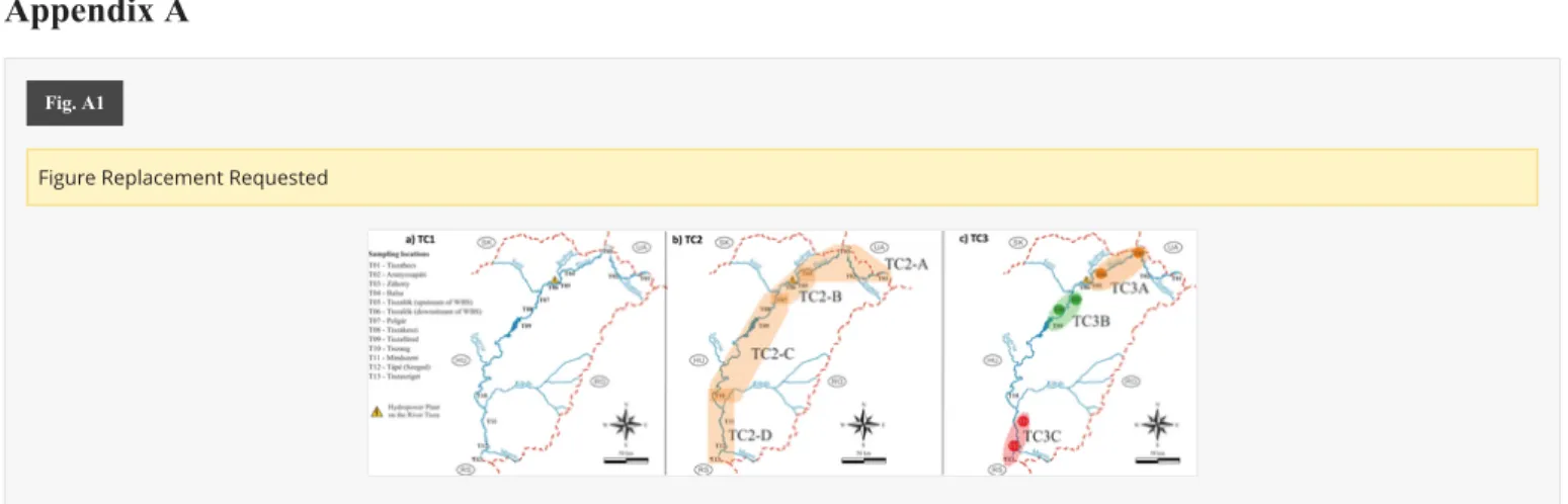
Illustration of the three different configurations: a) TC1 A), b) TC2 B) and c) TC3 C) used in the study. In TC 2 (B) the shaded backgrounds represent the sites used for training in the different setups, while in TC3 (C) these show the sites which were considered together for training and testing in the different setups. For details please see . Circles with similar colors in TC3 (C) show the homogeneous sampling sites determined in Tanos et al. (2015) .
Section 2.3
Replacement Instruction: Please replace the figure with the attached one! Thank you!
Fig. A2
Box-and-whiskers plots of A) water river runoff A) B) water temperature CB) pH DC) conductivity D) and E) dissolved oxygen E) at River Tisza sampling locations. Data falling outside a value of 1.5 times that of the interquartile range (outlying values) are indicated with a circle and those outside 3 times the interquartile range are marked with a redn asterisk (extreme values), the black lines in the boxes represent the median.
Table A1
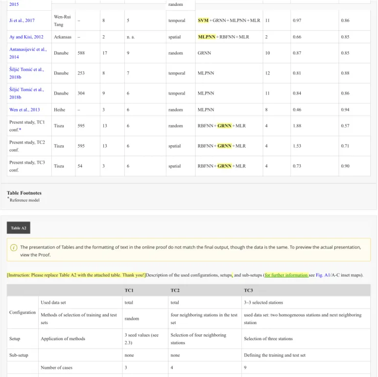
Results of dissolved oxygen estimation in literature and the present study. The selection column describes the way in which the training and test sets were divided, in which ‘temporal’ indicates an approach in which the ultimate time point(s) were used as the test set while ‘Spatial’ indicates the setup in which the test and training sets were chosen in a spatial manner using a combination of neighbouring sites. In the case of multiple models, the red ones highlighted in bold performed the best. Abbreviations: ANFIS: Adaptive neuro-fuzzy inference system, GRNN:
Generalized regression neural network, MLPNN: Multilayer perceptron; MLR: Multivariate linear regression, PLS2: Partial least squares regression, RBFNN: Radial basis function neural network, SVM: Support vector machine. The results from literature and the present study are both ordered in decreasing order of RMSE.
Reference River rkmRiver km
Sample points
Number of years
assessed Selection Models Input
parameters
Best RMSE (mg L-1) for the test set
Best R2 for the test set
Emamgholizadeh et
al., 2014 Karoon – 8 17 random ANFIS + MLPNN + RBFNN 9 3.15 0.85
Singh et al., 2009 Gomti 500 8 10 temporal MLPNN 13 1.23 0.76
Basant et al., 2010 Gomti 500 8 10 random MLPNN + PLS2 11 1.36 0.74
Bayram and Kankal, Harsit 143 9 1 controlled MLPNN + MLR 2 0.94 n.a.
i The presentation of Tables and the formatting of text in the online proof do not match the final output, though the data is the same. To preview the actual presentation, view the Proof.
Table Footnotes
Appendix B
Supplementary data
Supplementary data to this article can be found online at https://doi.org/10.1016/j.ecoleng.2019.07.023.
References
2015 random
Ji et al., 2017 Wen-Rui
Tang – 8 5 temporal SVM + GRNN + MLPNN + MLR 11 0.97 0.86
Ay and Kisi, 2012 Arkansas – 2 n. a. spatial MLPNN + RBFNN + MLR 2 0.66 0.85
Antanasijević et al.,
2014 Danube 588 17 9 random GRNN 10 0.87 0.85
Šiljić Tomić et al.,
2018b Danube 253 8 7 temporal MLPNN 12 0.81 0.88
Šiljić Tomić et al.,
2018b Danube 304 9 6 temporal MLPNN 11 0.84 0.86
Wen et al., 2013 Heihe – 3 6 random MLPNN 8 0.46 0.94
Present study, TC1
conf. * Tisza 595 13 6 random RBFNN + GRNN + MLR 4 1.88 0.57
Present study, TC2
conf. Tisza 595 13 6 spatial RBFNN + GRNN + MLR 4 1.53 0.71
Present study, TC3
conf. Tisza 54 3 6 spatial RBFNN + GRNN + MLR 4 0.73 0.90
*Reference model
Table A2
[Instruction: Please replace Table A2 with the attached table. Thank you!]Description of the used configurations, setups, and sub-setups (for further information see Fig. A1 /A-C inset maps).
TC1 TC2 TC3
Configuration
Used data set total total 3–3 selected stations
Methods of selection of training and test
sets random four neighboring stations in the test
set
used data set: two homogeneous stations and next neighboring station
Setup Application of methods 3 seed values (see 2.3)
Selection of four neighboring
stations Selection of three stations
Sub-setup none none Defining the training and test set
Number of cases 3 4 9
Notation TC1-A, TC1-B, TC1-
C TC2-A, TC2-B, TC2-C, TC2-D TC3-A#1, TC3-A#2, TC3-A#3, etc.
i The presentation of Tables and the formatting of text in the online proof do not match the final output, though the data is the same. To preview the actual presentation, view the Proof.
i The corrections made in this section will be reviewed and approved by journal production editor.
Abonyi, A., Leitão, M., Lançon, A.M., Padisák, J., 2012. Phytoplankton functional groups as indicators of human impacts along the River Loire (France).
Hydrobiologia 698, 233. doi:10.1007/s10750-012-1130-0.
Akkoyunlu, A., Altun, H., Cigizoglu, H.K., 2011. Depth-integrated estimation of dissolved oxygen in a lake. J. Environ. Eng. 137, 961–967.