ÓBUDA UNIVERSITY

(1)

ÓBUDA UNIVERSITY

A Thesis submitted for the degree of Doctor of Philosophy

A STUDY ON USING FIXED POINT TRANSFORMATION IN ADAPTIVE TECHNIQUES IN ROBOTICS AND

NON–LINEAR CONTROL Hamza Khan

Supervisor

Prof. Dr. habil. József K. Tar D.Sc.

Doctoral School of Applied Informatics and Applied Mathematics

August 19, 2020

(2)

Members of the Comprehensive Examination Committee:

Members of the Defense Committee:

Chairman:

Prof. Dr. Péter Nagy D.Sc., professor emeritus, Óbuda University Secretary:

Dr. Adrienn Dineva Ph.D. , Óbuda Universiy Opponents:

Prof. Dr. János Abonyi D.Sc., University of Pannonia Dr. Krisztián Kósi Ph.D., Óbuda Universiy

Further members of the Defense Committee:

Prof. Dr. László Szeidl D.Sc. professor emeritus, Óbuda University Prof. Dr. Róbert Fullér D.Sc., Széchenyi István University

Dr. György Cserey Ph.D., Pázmány Péter Catholic University

Date of the defense:

(3)

Declaration of Authorship

I, Hamza Khan, declare that the thesis entitled, “A Study on Using Fixed Point Transformation in Adaptive Techniques in Robotics and Non-linear Control”and the content presented in it, is entirely my own research work in the able supervi- sion ofProf. Dr. habil. József K. Tar. D.Sc.It is hereby assured that:

• This work has been completed as a candidate for Ph.D. degree at Óbuda University.

• Wherever in the thesis, the published work of other authors is consulted, this work is clearly referenced.

• Wherever in the thesis, quotations from other authors are used, then this fact is clearly mentioned. The thesis is absolutely my own work with the exception of such quotations.

• All the main sources of help have been properly acknowledged.

Budapest, 4 May, 2020.

Hamza Khan (Ph.D Candidate)

(4)

Dedication

To my dearest Father who is my mentor, leader and counselor, guided me in my childhood, encouraged and assured to be alongside of me every time. To my beloved Mother, her support, all time love and prayers provided me enough potentials in every step of life. To my Spouse, she sacrificed in the period of my Ph.D.

studies and patiently faced all hardships with courage and look after my beloved Muhammad Muzammil Hamza and Muhammad Hashir Hamza.

(5)

Acknowledgement

First of all, I am very thankful toAllah Almightywho helped me and provided the potentials to bear the hardships patiently and to be determinant in the complexities of life.

Secondly, my warmest gratitude goes to my respected supervisor Prof. Dr.

habil. József K. Tar D.Sc his all–time help, guidance, encouragement, and full support with his immense research skills pushed me up to this position where I am today and able to write this thesis. I am forever indebted to my supervisor, without his kind support it was impossible. He used to stand with me every–

time and provided tremendous knowledge using his all kind of expertise and research skills to make me able to complete my Doctorate Degree. Thank you, Sir.

I am also very thankful to the Doctoral School of Applied Informatics and Applied Mathematics, Óbuda University Budapest, Hungary, and all the faculty members on their full support in the past 4 years’ study period. Also, my warmest gratitude goes to the Tempus Public Foundationon providing all kinds of facilities during these years through the Stipendium Hungaricum Scholarship

& Dissertation Scholarship Programs.

My Special Thanks goes to my parents, teachers, friends, siblings, and all relatives who supported by any means. Especially I express my thanks to the International Office Mobility Department and its members, Obuda Student Hotel’s Authority to assisting all possible facilities during my time in Hungary, Europe.

Last but not least, my gratitude goes to the Hungarian Communities, during my stay they cooperated where I faced difficulties, their all–time cooperation will always be remembered.

(6)

List of Abbreviations

AF Auxiliary Function.

AMPC Adaptive Model Predictive Control.

ARHC Adaptive Receding Horizon Controller.

ASLRC Adaptive Slotine–Li Robot Controller.

CFAS Closed Form Analytical Solution.

CTC Computed Torque Control.

DoF Degree of Freedom.

DP Dynamic Programming.

FPI Fixed Point Iteration.

FPT Fixed Point Transformation.

GRG Generalized Reduced Gradient.

HOSVD Higher Order Singular Value Decomposition.

LHS Left Hand Side.

LMI Linear Matrix Inequality.

LPV Linear Parameter–varying.

LQR Linear Quadratic Regulator.

LTI Linear Time–invariant.

MPC Model Prdeictive Controller.

(7)

MRAC Model Reference Adaptive Control.

NFPT New Fix Point Transformation.

NP Non–linear Programming.

OC Optimal Controller.

PD Proportional and Derivative.

PID Proportional, Integral and Derivative.

PLC Programmable Logical Controller.

RFPT Robust Fixed Point Transformation.

RGM Reduced Gradient Method.

RHC Receding Horizon Controller.

RHS Right Hand Side.

SLARC Slotine–Li Adaptive Robot Controller.

T1DM Type 1 Diabetes Mellitus.

TP Tensor Product.

VBA Visual basic for Applications.

VS/SM Variable Structure – Sliding Mode Control.

(8)

Chapter 1 Introduction

The theory of controlling non–linear systems extensively was developed and used in the mid of the 20^th century and got more popularity with the passage of time.

A revolutionary change was seen after the invention of computer, that made this field easier especially when Rudolf Kálmán placed into the center of attention the state–space model formulated in the time domain instead of the frequency picture that was prevailing before the early sixties of the 20^thcentury [1,2].

In the most of the application areas within the frames of “Model Predictive Control” (MPC) [3,4] the controlled system’s dynamics (as a rigorous condition) mathematically is expressed as a “constraint” that has to be met while a “cost function” often representing contradictory requirements can be minimized with compromises. Among these compromises the limitation of the control force (caused by either the saturation of the drives or other reasons) can be taken into account. A possibility for tackling this problem is the method of “Dynamic Programming” (DP) that is based on the variation calculus and the resulting Hamilton–Jacobi–Bellman equation [5,6].

To evade the huge computational needs of the dynamic programming approach, in tackling the problems in the field of control the so–called non–linear programming approach can be applied. The heuristic “Receding Horizon Controllers” (RHC) that were introduced for industrial use in the seventies of the past century [7] approximate the (MPC) over a finite time–horizon by the use of an available approximate dynamic model only, and for the compensation of the consequences of the modeling imprecisions and unknown external disturbances, the controlled system’s state is directly observed or estimated by the use of observable data in the last point of the horizon that can be used as a starting point of the next one. Normally, the finite horizon is approximated by a discrete time–grid, and nonlinear programming is used for the calculation of the solution

(11)

in which the solution is computed by the use of Lagrange’s “Generalized Reduced Gradient” (GRG) method published in 1811 [8].

Usually, replacing a non–linear system by a simple linear one is considered as a simple and effortless way to find the approximate solutions whenever it is satisfactory to consider the system’s operation in the vicinity of a “working point”. In this narrow vicinity the system can be approximated as a “Linear Time–Invariant” (LTI) one. Sometimes this approximation well captures the system’s dynamics e.g. in modeling the behavior of the air path of Diesel engines [9]. In the close vicinity of a “working point”, the traditional control design approaches that were based on the properties of the “Linear Time–Invariant”

(LTI) systems by using the frequency domain, linear integral transformations as the Fourier, Z, or Laplace transforms [10], can lead to satisfactory results.

However, in many cases linearization (called “affine approximation”) cannot be a relevant and satisfactory way in approximating the controlled system’s dynamical model. Often a “system switching” has to be tackled between the neighboring cells of the state space that contain the localLTI models [11]. This approach has been extended in the tracking control for switched linear systems with time–varying delays [12,13].

In other approaches the so called “Tensor Product Control Models” (TP) can be used based on polytopic dynamic models, “Higher Order Singular Value Decomposition” (HOSVD), and “Linear Matrix Inequalities” (LMI) as e.g. in [14, 15, 16]. This branch of research typically is based on the possession of a reliable complex system model that in the first phase is transformed into a TP form “offline” by the use of a computer. In the second step the “unnecessary complexity” of this transformed model is reduced by the application ofHOSVD.

Finally, according to the program announced by Boyd et al. in 1994 in [17], the so obtained model’s control can be systematically tackled by existing software algorithms based on the use ofLMIs.

It has to be emphasized that though the “heuristic RHC” provides a quite wide framework for control approaches, it suffers from some limitations that seem to be crucially significant in engineering applications. In the case of using general forms for the cost functions and allowing the use of arbitrary nonlinear models no rigorous statements can be done on the nature of the obtained solutions. Due to the fact that the number of the Lagrange multipliers equals with that of the state variables in the constraint terms, these state variables and their associated Lagrange multipliers behave like the canonical variable pairs of Classical Me- chanics [18]. Consequently an “artificial Hamiltonian” can be associated with the

(12)

realized “optimal motion”, and this Hamiltonian is kept constant. Furthermore, in the tangent space of these “canonical state variables” the rules of the Symplectic Geometry are valid that means that the “volume” of the phase cells remains constant (Liouville’s Theorem in Classical Mechanics), i.e. the motion is similar to the flow of some incompressible fluid (that also satisfies complementary conditions regarding the partial derivatives according to the control forces). In general, “incompressibility” does not promise very nice numerical behavior for the solutions. If in certain direction the cells are shrunk, in other directions they have to be extended to save their volume. This concerns stability issues: it cannot be expected that the solution can be settled in an attractive point of the state space. On this reason in the practice the otherwise quite wide frames of the RHC controllers are applied under strictly “narrow” conditions as follows:

a) Normally the cost functions are quadratic terms constructed of constant symmetric positive definite matrices and the state tracking errors. Con- sequently, their derivatives in the reduced gradient method will be well behaving linear functions of the tracking errors.

b) Generally similar quadratic terms are in use for the limitation of the control forces that provides similar advantages.

c) In the case of LTI system models the Lagrange multipliers can be constructed as the product of some symmetric matrices and the state variables.

The equations of motion for these matrices can be decoupled from that of the state variables, that is a great advantage.

d) The equations of motion obtained for these matrices satisfy some Riccati equation with some “terminal condition”. In the 18^th century Riccati realized that special first order quadratic differential equations can be solved by obtaining the solution for linear, second order differential equations [19].

Therefore, under these special conditions certain “general view” of the solution became available. The matrix versions of the Riccati equations obtained wide scale use in control technology (e.g. [20,21]).

e) Regarding certain constraints, Schur’s matrix complement [22] can be applied to transform quadratic constraints into linear ones that can be efficiently tackled by theLMItechniques as it was recommended by Boyd et al. in [17].

One of my main aims was to “liberate” the researchers from the above restrictions in theRHCcontrol by the application of non–quadratic cost functions

(13)

that for instance can “better tolerate” smaller errors and “more drastically punish”

greater ones than a simple quadratic structure.

It was considered an open question since a few years ago that the combination of theMPC within the frame of “Optimal Controllers” with some adaptive techniques can be possible in the area of control theory.

In the field of control theory to design non–linear adaptive controllers, generally Lyapunov’s well known 2^nd or “Direct Method” [23, 24] is used. It is widely applicable in recent days, too. But its typically complex design process is considered as burden and difficult, therefore alternative simple methods were adopted. It has the great advantage that it provides a basis to design traditional and classical non–linear controllers. The purpose is to concentrate on the problem of the stability of the motion of the controlled non–linear system. Though, this has great advantages in the related field but despite those excellent advantages, the Lyapunov function–based approach suffers from certain disadvantages, too. Beside the fact that this method needs tricky and complex mathematical designer’s skills, it typically prescribes rather “satisfactory” than “necessary and satisfactory” conditions in the proofs. Consequently it allows the application of a huge set of possible control parameters that maintain the stability and in the same time crucially influence the transients of the controlled motion without any optimization.

To get rid of the very complicated Lyapunov function–based adaptive solutions in 2009 an alternative approach “Fixed Point Transformation” (FPT) was proposed [25] where, the problem at first was transformed into the fixed point task and then the idea of iteratively finding the fixed–point of a contractive map was used. This idea is based on Banach’s well known Fixed Point Theorem [26].

In my research the said idea was further extended regarding new aspects where the approach was combined with other methods and also was applied to get rid of the complicated burden of the precise calculation of the Jacobian in the inverse kinematics of robots. The purpose, also, is to give some contributions and achievements in this new line of problem tackling in adaptive control. I am especially interested in the possible combination of the traditional and the novel approaches.

1.1 Research Aims in the Mirror of the State of the Art

This is the era of modern sciences and technologies. Things and technologies continuously keep changing due to new ideas and up–to–date technological

(14)

instruments. Such ideas and the advanced technological revolution bring severe changes in several natural systems in the Universe. Abundant of systems are there in the Universe, based on non–linear functional dependencies. Their non–

linearity was always considered a great challenging subject for the researchers in view of their stability and efficient control. The control of such systems, by numerous techniques, fall in the area of study named “Control Theory”.

To deal with such systems only a few methods were used before the last decade of the 19^th century but later in 1892 Alexander Lyapunov elaborated his way of solution in his doctoral dissertation to deal with the stability of the systems giving his theory with the approach named as “Lyapunov’s Direct or Second Method” to determine the stability of a non–linear system without solving its equations of motion.

It is evident that, a control designer tries to bring about better and efficient methods to maintain the stability of the controlled systems. In the beginning, getting the solutions of the problems, based on non–linearity, were very hard due to the fact that only “manual working system” (consisting of crank driven mechanical calculators, slide–slip, metric paper and the tabulated form of certain special functions) was available, but later the invention of the computers provided an easy way to proceed in this area of study to extend it and widen its view from different aspects.

To understand the working process and criteria of the systems, consideration of their modeling and controlling process, measuring or estimating the states of the systems efficiently have become the prime need of the time. For the purpose of controlling the systems and to understand their stability, different varieties of methods and terminologies have been used in different times to enrich the stabilities.

Adaptive control is one of the methods where a system uses the techniques and approaches to change itself according to the behavior in new or varying circumstances. The motivation to consider this area of study was gotten in early fifties of the previous century when an autopilot high performance based aircraft for high altitudes and wide range of speed was designed. After this approach the study area got more attention in all aspects of life. Examples for a quite rich variety of problems in practical life can be mentioned in this context: the glucose–insulin metabolism [27, 28, 29, 30, 31, 32], the pharmaco–kinetics of various drugs in anaesthesia [33, 34, 35, 36], modeling the operation of the neurons and the nervous system [37, 38, 39, 40, 41] in life sciences, dynamic models of robots [42, 43], chemical processes like crystallization [44], efficient

(15)

control of freeway traffic [45, 46,47] including the limitation of the emission of polluting materials [48,49], etc. can emphasize its importance and applicability.

The study of adaptive techniques for non–linear systems has considerable mathematical difficulties. Analyzing them theoretically is, in fact, a very complex and hard task. Therefore, the modern techniques and approaches in view of approximations in control design and signal processing include a various class of mathematical tools.

In the last decade of the 20^th century the idea ofMPCwas vastly investigated (e.g. [50, 51]), and its novel developments (e.g. [4]) were successfully used in different fields of the life as e.g. in chemistry [52,53,54,55], life sciences–related problems [56], economy [57], etc. Another use of advanced control solutions is, to get attention in today’s medical practice regarding the control of physiological processes [58]. Many control solutions are under development which can be used for various kinds of control problems. It has been observed that there are many advanced control methods that have been successfully applied for physiological regulation problems, for example control of anaesthesia [59, 60], antiangiogenic inhibition of cancer [61, 62], immune response in presence of human immunodeficiency virus[63] and regulation of blood glucose (BG) level [64,65,66,67] as well.

In the applications the non–linear nature of the advanced control techniques have high importance. Beside the non–linearities in the control problems the researchers on the field are facing with many challenges such as model and parameter uncertainties and even time–delay effects, too.

It is well known that in designing the adaptive controllers, based on the non–linear systems mostly Lyapunov’s “direct” or “second method” is applied as a traditional approach [23, 24]. Essentially the same approach is extended to tackling time–delay problems by the use of the Lyapunov-Krasowskii functional [68]. The complexity of this method diverted the attention of researchers to propose the alternative simple approaches (e.g. [69, 70, 71, 72]). According to the basic facts the work of Lyapunov’s method can be summarized as follows [73]:

a) it can be used to create the satisfactory conditions to guarantee the stability, b) it does not focus on the tracking error relaxation in the initial phase of the controlled motion, but provides the opportunity to prove the global stability that is very necessary in common cases,

(16)

c) in the case of certain adaptive approaches for the identification of the parameters of the model of the controlled system, it provides significant methods, d) it works with a large number of arbitrary adaptive control parameters because it contains certain components of the particular Lyapunov function in use, and may require further parameter optimization (e.g. [74]).

It is realized that the mathematical framework of the traditional MPC can hardly be combined with the Lyapunov function–based adaptive control. Certain approaches combining MPC and Lyapunov’s stability theorem can be found in the literature (e.g. [75,76]).

Concentrating on the primary design intent the “Robust Fixed Point Trans- formation” (RFPT)–based technique was suggested in which the non–linearly optimized trajectory can be adaptively tracked iteratively by the adaptive controller that converges to the appropriate point, based on Banach’s Fixed Point Theorem [26]. Furthermore, the suggested “adaptive, iterative inverse kinematic approach” [77] – based on [78, 79] – can be convergent and useful even if the Jacobian of the robot arm is only approximately known. The application of an “abstract” rotational transformation in the state space can improve the convergence properties of the iteration without the need for obtaining complete information on the actual (i.e. the “exact”) Jacobian. It is just enough to utilize the simple motion steps generated by the iteration that produces a smooth motion.

Similarly, a possible recent improvement of theRHC approach was reported in [80] that corresponds to the adaptive tracking of the optimized trajectory instead of exerting the forces calculated by the optimization algorithm on the basis of an available, approximate dynamic model.

All the above discussed results are introduced in our papers published recently (e.g. [80, 81, 82, 83], [84], [85], and [86], [87]). The main directions for this research will be outlined in the next section.

1.2 The Structure of the Thesis

The possible application and possible improvement of the Classical “Receding Horizon Controller” (RHC) and its application has been discussed in Chapter2in details.

(17)

In the initial stage the possibilities and useful applications of the design of the Classical RHC by using Non–linear Programming (NP) was investigated.

After that, using the Generalized Reduced Gradient method, to overcome the complexities of non–linear optimization task the study was further extended to deal with the Type 1 Diabetes Mellitus, one of the dangerous disease for humanity, that needs treatment in the form of control. To check the performance of the solution “soft” disturbance and “unfavorable” disturbance signals were applied and studied.

To improve and overcome the disadvantages and difficulties in the field of non–linear control, a novel “Fixed Point Transformation” (FPT) recently invented by A. Dineva in [88, 89] was applied by combining it with the classical RHC.

The alternativeFPTapproach was so introduced in adaptive control that, instead of Lyapunov’s “2^nd Method”, it was based on Stefan Banach’s “Fixed Point Theorem”. This method was applied in various aspects to achieve precise and meaningful results. The combination of this method with theRHCis based on the idea that in the classical optimal control both the state variables and the control signals are estimated for the horizon based on the approximate dynamic system model. However, instead of exerting the so obtained control signals, the system adaptively tries to track this “optimized trajectory”. For making simulation examples a simple 1^storderLTIsystem was investigated in the adaptive control.

In Chapter3the adaptiveRHCis explained for some special problem classes that are directly treatable by the use of the “Auxiliary Function” (AF).

In Chapter 4 the “Inverse Kinematic Task of Robots” is adaptively solved using the FPT method. It has been observed that in a wide class of robots of open kinematic chain the inverse kinematic task cannot be solved by the use of closed–form analytical formulae. On this reason the traditional approaches apply differential approximation in which the Jacobian of the “normally redundant”

robot arm is “inverted” by the use of some “generalized inverse”. These pseudo–

inverses behave well whenever the robot arm is far from a singular configuration.

However, in the singularities and nearby the singular configurations they suffer from a singular or ill–conditioned pseudo–inverse. For tackling the problem of singularities normally complementary “tricks” have to be used that so “deform”

the original problem that the deformed version leads to the inversion of a well–conditioned matrix. Similarly, in the inverse kinematic tasks in robots the burden of the typical computations of Jacobian were removed by using the FPT via JULIA and MATLAB simulations.

Chapter 5 is the “conclusion chapter” where all the related novelties of this

(18)

thesis will be discussed briefly. Finally, in Chapter 6 the study is discussed in future prospects that what results and novelties are being expected? Also, how we will be able to achieve reliable results according to the topic of the thesis?

1.3 Research Methodology

It is obvious that the computational mathematical problems and engineering topics need simulation–based studies to understand and further extend the existing solutions. The wide range of practical problems results in differential equations that cannot be solved analytically, can be studied via numerical methods using simulations and programming. Such problems can be applied and understood after the validation of the simulation investigations. For this purpose a lot of mathematical packages can help to find the clear results.

In the period of my study, I used the JULIA Programming Language for the programming purposes to find the required results of my research. It provides an easy, simply coded and fast running programming possibility. Similarly, the simple VISUAL BASIC of MS–EXCEL 2010 was also used that helped to easily compile the results by simple programming. In some cases I used Matlab 2018, too, to find the results easily. Matlab is a heavy but precise programming language which helped in rare cases to easily go through from my work.

The JULIA Package developed under the MIT and GPLv2license works by providing a modeling and computational interface for solving the dynamical problems. Julia is a high–level, high–performance dynamic programming language developed specifically for scientific computing [90]. This dynamic language ensures a very fast evaluation for technical computing. The applied scientific methods en- sure the precision and thoroughness of the simulation results. It has an ability for distributed parallel task execution. It also has numerous developer communities who made some “extra” packages with the use of the build–in package manager.

At its official website [90], the main features of the language are mentioned as

• Multiple dispatch: providing ability to define function behavior across many combinations of argument types

• Dynamic type system: types for documentation, optimization, and dispatch

• Good performance, approaching that of statically–typed languages like C

• A built–in package manager

(19)

• Lisp–like macros and other meta–programming facilities

• Call Python functions: use the PyCall package

• Call C functions directly: no wrappers or special APIs

• Powerful shell–like abilities to manage other processes

• Designed for parallel and distributed computing

• Coroutines: lightweight green threading

• User–defined types are as fast and compact as built–ins

• Automatic generation of efficient, specialized code for different argument types

• Elegant and extensible conversions and promotions for numeric and other types

• Efficient support for Unicode, including but not limited to UTF–8

For the research concerning optimization programs, a developed simple program in “Visual Basic for Applications” (VBA) in the background of the MS EXCEL serves as an excellent solution provided that the size of the problem is not too big.

The MS EXCEL’s “Solver” module is provided by an external firm (Front–line Systems, Inc.). There are various solutions implemented into the Solver module, including the “Generalized Reduced Gradient” (GRG) method which can be used in the given case as well. TheGRGis based on [91,92] and its usability has been proved in various fields of research as e.g. in [83]. The problem conveniently can be formulated by functional relationships between the contents of the various cells of the worksheets. For this purpose User Defined Functions can be created in VBA. Then for the Solver a “model” can be specified by giving the cell that contains the cost to be minimized, the location of the independent variables and the constraints in the worksheets, and the parameter settings of this optimization package. The so defined “model” can be saved somewhere in one of the worksheets. Following that a small program can be written inVBA that declares the model parameters as global variables, reads their actual values from the worksheets, loads the “model” for the Solver, and for the horizons under consideration cyclically:

a) fills in the cells with the data of the nominal trajectory to be tracked, the initial values of the variables to be optimized, and the control forces,

(20)

b) calls the Solver with the options that it must stop optimization if the pre- scribed limits in the time or step numbers have been achieved, keeps the so obtained results, and

c) writes the optimized results in certain cells of a worksheet that are used for making various graphical representations of the results.

Regarding the “reliability” of the computed data, because we investigated

“convergent iterations” in the simulation programs, the key factor was the time resolution of discretization. After obtaining certain numerical results with a given fixed time–step ∆t, the same computations were repeated with .×∆t.

If no observable differences in the results were observed, the computation was regarded as “reliable result”. Roughly speaking, this practice corresponds to stopping an iteration when the subsequent variations in a convergent Cauchy sequence become small enough. In the practice such solutions are prevailing.

In the Julia realizations I applied the simple Euler integration in sequential programs. This structure was treatable in this manner. In the case of optimization programs, the role of∆t corresponded to the discrete time resolution in the case of Non–linear Programming. These problems were also treatable in this manner. I have to note that the problems in the convergence were influenced by other parameters in the Solver’s setting as e.g. the maximum number of numerical steps or the maximal time allowed for finding the optimum. The effects of these parameters were separately considered in the programs realized by the EXCEL–VBA–Solver combination.

(21)

Chapter 2 Improvement of the Classical

Receding Horizon Controller and Its Applications

In industries, for more advanced controlling purposes, the vastly applicable heuristic Receding Horizon Controller (RHC) invented in 1978 [7] can be used.

By using the best possibilities of the RHC we are able to predict the possible future behavior of our system, moreover, we are able to intervene in its operation as well. I have investigated the possibilities of the design of a Receding Horizon Controller by using Non–linear Programming to simulate a possible treating for patients suffering from Type 1 Diabetes Mellitus [A. 1]. The non–linear optimization task was solved by the Generalized Reduced Gradient (GRG) method.

Diabetes Mellitus (DM) is the collective name of several chronic diseases connected to the metabolic system of the human body. There are many types of DM. The most dangerous is the Type 1 DM (T1DM) where the metabolic system is not able to function normally due to the lack of insulin. Type 2 DM (T2DM) which is the most widespread kind of DM and it occurs mostly because of the lifestyle. In this case the usual is that the blood glucose and insulin levels are continuously increasing over a long period of time. Due to the extreme glucose and insulin load, the cells are becoming resistant to the insulin over time. In order to compensate this condition the body produces more and more insulin – which leads to the “burnout” of the pancreaticβ–cells which produce the hormone. At this point the T2DM turns into T1DM. Other frequently occurring type is the Gestational DM (GDM ) from which women may suffering during pregnancy.

Usually, this condition is temporary, however, sometimes it turns into T2DM and becomes permanent [93,94,95].

(22)

The investigations were done on the basis of a particular system model, the

“Modified Minimal Model” [96] which originates from the model of Bergman [97]. Two practically important scenarios were investigated. In the first one, I applied “soft” disturbance – namely, smaller amount of external carbohydrate – in order to be sure that the proposed method operates well through the optimization process. In the second scenario, “unfavorable” disturbance signals were applied – a highly oscillating, peak kind external excitation with cyclic nature.

I have found that the performance of the realized controller was satisfactory and it was able to keep the blood glucose level in the desired healthy range – by considering the restrictions against the applicable control action.

In the 2^nd step, as a preliminary investigation, I studied the possibility for the adaptive extension of the RHC method in combination with the Fixed Point Transformation–based approach [A.2]. In this case the simplest 1^st order 1 DoF LTIsystem model was used. The combination of this method with the Receding Horizon Control is based on the idea that in the classical optimal control both the state variables and the control signals are estimated for the horizon based on the approximate model using Lagrange’s “Reduced Gradient Method” (RGM).

It provides the “estimated optimal control signals” and the “estimated optimal state variables” over this horizon. The controller exerts the estimated control signals but the state variables develop according to the exact dynamics of the system.

I have used the suggested alternative approach in which, instead of exerting the estimated control signals, the estimated optimized trajectory is adaptively tracked within the given horizon. Simulation investigations are presented for a simpleLTI model with strongly non–linear cost and terminal cost functions. In this investigation I found that the transients of the adaptive controller that appear at the boundaries of the finite–length horizons reduce the available improvement in the tracking precision. In contrast to the traditionalRHC, in which decreasing horizon length improves the tracking precision, in my case some increase in the horizon length improves the precision by giving the controller more time to compensate the effects of these transients.

(23)

2.1 Scientific Antecedents

Regardless of the type of DM a few common control goal can be defined: keep the glycemia (the BG level) in the healthy range; total avoidance of hypoglycaemic periods; and avoid the high BG variability as far as possible [98,99,100].

In case of T1DM many solutions are available, however, all of them have their own limitations, simplifications and restrictions – thus, none of them are general [67]. In these days from control point of view the most beneficial approach is the Artificial Pancreas (AP) concept. This idea aims to imitate the regular working of the pancreas from the insulin production point of view, namely, administering insulin demands on the needs determined by the BG level [101]. Thus, we have to face with contradictory requirements: the generalization and personalization as well.

One of the mostly used algorithms is the modified proportional–integral–

derivative (PID) based solutions due to their simplicity and flexibility. Moreover, several clinical trials have been done by using these methodologies and investigated their effectivity [102, 103, 104]. Linear Parameter Varying (LPV) based solutions have high importance, since, the uncertainties can be handled with high efficiency by them [66,64, 105]. The Tensor Product (TP) based techniques also represent interesting directions, since, they can be combined by Linear Matrix Inequality (LMI) based control and LPV methodology as well [106, 107, 65].

The most frequently used method is the Model Predictive Control (MPC) with regard to the control of DM [108,101,109].

By its applicability and persistency MPCapproach is widely used in various research fields as well [44, 110, 57]. In general the goal of theMPCapplications is the tracking and stabilization [111].

The RHC framework can be hardly combined with the Lyapunov function based control. However, certain approaches can be found in the literature where the Lyapunov stability and RHC was successfully combined for specific cases [75, 112]. Alternative solutions also exist which can be used instead of Lyapunov’s stability theorem. The “Robust Fixed Point Transformation” (RFPT) based control [25, 113] uses Banach’s fixed point theorem [26] to transform the control task into a fixed point problem which can be solved iteratively. This method allows to design a robust iterative adaptive controller which can avoid the main limitations ofRHCif these are combined.

(24)

2.2 Investigation of the Applicability of RHC in Treating the Illness Type 1 Diabetes Mellitus

During my research I have applied a modified Minimal Model [96] which originates from the model of Bergman [97]. This model has several beneficial properties, such as simplicity, good transformability, flexibility and it is based on simpler biological considerations. The main goal of the model is to describe the glucose–insulin dynamics, namely, to define the connection between the blood glucose and insulin levels. Although, in order to characterize the daily life of aT1DMpatient by the model, it is needed to extend it with additional sub–models.

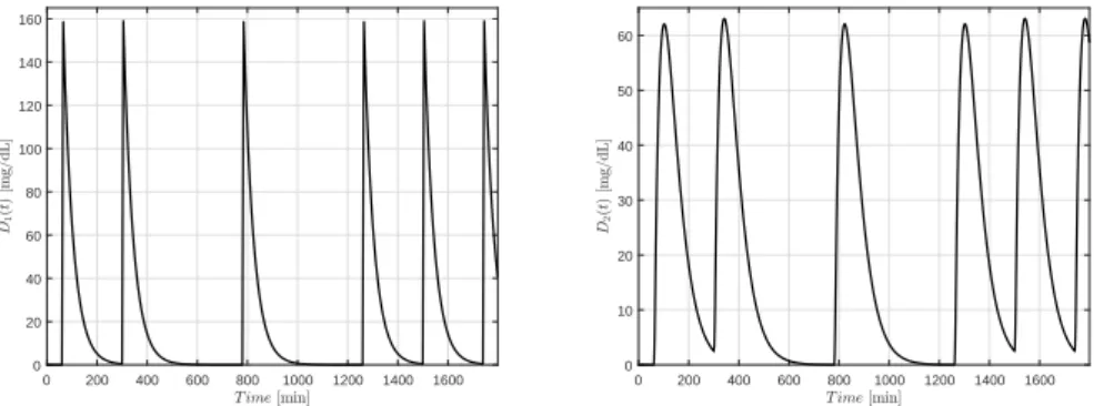
These sub–models are the absorption of the external glucose and insulin intake. During the daily routine these substances are not directly injected to the blood stream – however, this can occur in case of persistent hospitalization – instead the carbohydrate is consumed via food intake and the insulin is entered through the extracellular tissue matrix under the skin [93]. Thus, the characteristic of their appearance in blood has rather peak kind than elongated dynamics. The glucose and insulin absorption is described by (2.1) – (2.4), respectively. These sub–models are coming from the Cambridge model [114], but I applied them in appropriate dimensions to insert it to the core model. The core model is described by (2.5) – (2.7).

D˙_(t) = − 

τ_DD_(t) +A_g

M_wGV_GC·d(t), (2.1) D˙_(t) = − 

τ_DD_(t) + 

τ_DD_(t), (2.2)

S˙_(t) = − 

τ_SS_(t) + 

V_Iu(t), (2.3)

S˙_(t) = −

τ_SS_(t) + 

τ_SS_(t), (2.4)

G(t) = −(˙ p_+X(t))G(t) +p_G_B+ 

τ_DD_(t), (2.5) X˙(t) = −p_X(t) +p_(I(t) −I_B), (2.6)

I(t) = −n(I(t) −˙ I_B) +  τ_S

S_(t), (2.7)

(25)

The meaning and purpose of the state variables in (2.1) - (2.7) are as follows:

D_(t) mg/dL and D_(t) mg/dL are the primary and secondary compartments belonging to glucose, where τ_D time constant determines how long it takes the meal is absorbed after consumption in time. S_(t) mU/L and S_(t) mU/L are the primary and secondary compartments belonging to insulin, where τ_S time constant determines how long it takes the insulin absorbed after injection (to the extracellular space) in time. The G(t) mg/dL is the blood glucose (BG) concentration – the so–called glycemia –,I(t)mU/L is the blood insulin concentration and X(t) 1/min is the insulin-excitable tissue glucose uptake activity – which describes the connection between the blood’s glucose and insulin levels, respectively.

From system engineering point of view the external glucose, namely, the food intake can be handled as disturbance. In this case d(t) g/min is the disturbance input. It can be inserted to the D_(t) via the (A_g)/(M_wGV_G)

C complex which describes the bio-availability of the glucose from complex carbohydrates.

The u(t) mU/min control signal – the injected insulin – is directly connected to S_(t). More detailed description of the used model parameters can be found in Table2.1and in [96,114].

Table 2.1: The applied parameters of the models in this study [96,114,115].

Notation Value Unit Description

G_B  mg/dL Basal glucose level

I_B . mU/L Basal insulin level

p_ . /min Transfer rate

p_ . /min Transfer rate

p_ . L/(mU min) Transfer rate

n . /min Time constant for

insulin disappearance

BW  kg Body weight

V_I .BW L Distribution volume of insulin

V_G .BW L Distribution volume of glucose

M_wG . g/mol Molecular weight of glucose

A_g . − Glucose utilization

C . mmol/L Conversion rate between

mmol/Landmg/dL

τ_D  min Carbohydrate (CHO) to glucose

absorption constant

τ_S  min Insulin absorption constant

(26)

2.2.1 Simulation Results for Treating T1DM with RHC

During the development of the appropriate cost function – which fits to the given problem – the specificities of the model (2.1) – (2.7) should be taken into account. The main limitation coming from the model is the amount of injectable insulin and the fact that I do have only one control signal. Due to the applied control signal instances from the given horizon are independent variables in the optimization problem applying a specific form of limitation on them – a “bias”

– is reasonable. Thus, the control signal in this construction should be limited in accordance with the phenomenon to be controlled. Further, not the control signal itself, but another variable should be selected as independent variable to avoid the initial value problems causing the rough numerical approximation at the beginning of the optimization. This is caused by the high non-linearity in the model.

Another property of the model that only theG(t)blood glucose level can be measured. Thus, only this state variable can be embedded into the cost function to be developed. I do not have internal information about other state variables of the process to be controlled during action – which is the internal operations of a human being –, namely, this limitation has to be taken into account. Due to such reasons I have applied a more specific cost function defined in (2.8):

{xmin, ...,x_F} {u...,u_F_−}

F−X

i=

J(x_i,u_i) +Φ(x_F)

subject to x_i+−x_i

∆t −f(x_i,u_i) =0,

(2.8)

and{λ, . . . ,λF−}are the Lagrangian multipliers – which are used in accordance with the optimization task to be solved by the reduced gradients method.

{Gmin, ...,GF} {v...,vF−}

F−X

i=

J(G_i,u_i) +Φ(G_F)

subject to x_i+−x_i

∆t −f(x_i,u_i) =0

, (2.9)

whereu_i=u_bias+tanh(v_i). We have developed a strongly non-linear cost function in which all requirements can be embedded against the control action to be reached during control.

J(G,u)^{de f}=

G^N−G A_

α

+B

u A_

α

, (2.10)

(27)

Φ(G_F)^{de f}=

G^N_{f inal}−G_{f inal} A_

α

. (2.11)

The tracking error in (2.10)–(2.11), namely, the deviation of the realized blood glucose level G(t) from the nominal blood glucose level G^N(t) can be calculated asG^N_i −G_iat the grid points. The absolute value of this difference can be determined byA_ and A_ parameters which contribute the belonging level of

“penalty” prevails in the cost function. In that case if α>  andα>  beside

|G^N−G|<A_and|G^N_{f inal}−G_{f inal}|<A_, then the contribution to the cost function is low. However, if|G^N−G|>A_and|G^N_{f inal}−G_{f inal}|>A_then due to the power terms the contribution to the cost of these terms are drastically increasing. The α_ and α_ constants can be used for different purposes. α_=α_ = provides proportional contribution, namely, the pure deviation will be better prohibited.

Although, if α,α < , then the smaller deviations will be prohibited better than the bigger ones. The role of the A_ andα_ parameters are similar, namely, the applied control input can be prohibited by applying them. TheB parameter allows to modify the enforcement of the effect of the control signal in the cost function.

In order to test the realized control framework I investigated two scenarios. In the first scenario 25 g CHO was considered – 5 g over 5 minutes in each 240^th time instance from the 60^th time instance. In the second scenario we considered 50 g CHO intake – 10 g over 5 minutes in each 240^th time instance from the 60^th time instance. In both cases 200 time horizons have been considered within 10 grid points, thus the total simulated time domain was 2000 minutes. The resolution∆twas 1 minute in accordance to the properties of the model.

The applied cost function parameters (which represent the control parameters in this regard) can be found in Table 2.2. It should be noted that I have used permanent reference trajectories in both cases denoted by G^N = 90 mg/dL in (2.9)–(2.11).

Therefore, in accordance with the aforementioned details, the goal of the control becomes to keep theG^N = 90 beside respecting the predefined u_bias. In this manner – via the cost function – the deviations from these predefined values have been “punished”, namely, the value of the cost function became higher.

(28)

Table 2.2: The parameters of the applied cost function (2.10).

Scenario 1 Scenario 2 A_ mg/dL mg/dL

α  

A_ mU/min mU/min

α_  

A_ mg/dL mg/dL

α  

u_bias mU/min mU/min G^N mg/dL mg/dL

2.2.1.1 Results of Scenario 1

In the followings the results of Scenario 1 are presented. First, the disturbance signal is shown by Left Hand Side (LHS) of Fig. 2.1. The applied – calculated – control signal can be seen on Right Hand Side (RHS) of Fig. 2.1. It is clear that the controller is able to administer the insulin in accordance to (2.9)–(2.11) where theu_i=u_bias+tanh(v_i)is prevailed in the control action.

Figures 2.2 show the absorption of glucose and its appearance in the blood with the dynamics determined by the model. Figures2.3show the absorption of insulin from the interstitium and its appearance in blood.

0 200 400 600 800 1000 1200 1400 1600 0

0.5 1 1.5 2 2.5 3 3.5 4 4.5 5

0 200 400 600 800 1000 1200 1400 1600 0

5 10

0 5 10 15 20 25 30 35 40

0 5 10

Figure 2.1: Applied disturbance (CHO intake) – 5 g over 5 minutes at each 240^th time instance (LHS) and the calculated control signals (RHS). The upper figure represents the whole time horizon. The lower figure shows a piece of the whole time horizon between 0 and 40 minutes.

(29)

0 200 400 600 800 1000 1200 1400 1600 0

20 40 60 80 100 120 140 160

0 200 400 600 800 1000 1200 1400 1600 0

10 20 30 40 50 60

Figure 2.2: Variation of the first (LHS) and second (RHS) states of the glucose absorption subsystem.

0 200 400 600 800 1000 1200 1400 1600 0

5 10 15 20 25 30 35

0 200 400 600 800 1000 1200 1400 1600 0

5 10 15 20 25 30 35

Figure 2.3: Variation of the first (LHS) and second (RHS) states of the insulin absorption subsystem.

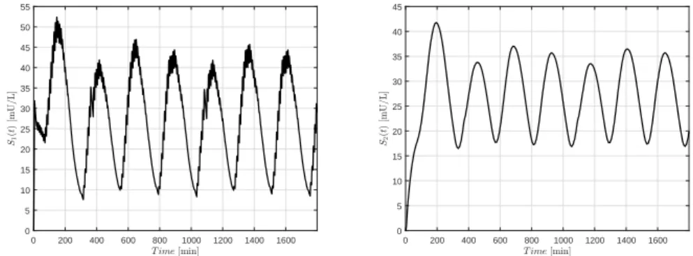
The main point can be seen on Fig. 2.4. The controller is able to satisfy the determined conditions and the BG level (G(t)) is inside the predefined range – no hypo- and hyper-glycemia occurred. The BG level approaches the selected reference trajectory (G^N) as it is expected.

On Figs. 2.5 the the variation of blood insulin level and intermediate state variable can be seen. X(t) determines how the blood insulin level affects the blood glucose level, namely, the connection between them.

(30)

0 200 400 600 800 1000 1200 1400 1600 80

100 120 140 160 180

Figure 2.4: Variation of the blood glucose level over time

0 200 400 600 800 1000 1200 1400 1600 0

0.5 1 1.5 2 2.5 3 3.5 4

0 200 400 600 800 1000 1200 1400 1600 0

0.002 0.004 0.006 0.008 0.01 0.012

Figure 2.5: Variation of insulin levels and variation of the insulin-excitable tissue glucose uptake activity over time

2.2.1.2 Results of Scenario 2

The applied disturbance input in accordance with the detailed protocol can be seen onLHSof Figure2.6. In this case, we have applied higher inputs in order to be sure that the developed control framework is able to deal with unfavourable external excitation.

Figure2.6. (RHS) is the calculated and administered control signal. As it is visible, the dynamics of it is significantly different than the previous case due to the different settings in the applied cost function.

Figures 2.7. represent the absorption of the glucose and its appearance in the blood with the dynamics determined by the model. Figures 2.8. show the absorption of insulin from the interstitium to the blood.

(31)

0 200 400 600 800 1000 1200 1400 1600 0

1 2 3 4 5 6 7 8 9 10

0 200 400 600 800 1000 1200 1400 1600 0

20 40

15 20 25 30 35 40 45 50

0 5 10

Figure 2.6: Applied disturbance (CHO intake) – 10 g over 5 minutes at each 240^th time instance (LHS) and the calculated control signals (RHS). The upper figure represents the whole time horizon. The lower figure shows a piece of the whole time horizon between 0 and 40 minutes.

0 200 400 600 800 1000 1200 1400 1600 0

50 100 150 200 250 300

0 200 400 600 800 1000 1200 1400 1600 0

20 40 60 80 100 120

Figure 2.7: Variation of the first (LHS) and second (RHS) states of the glucose absorption subsystem.

0 200 400 600 800 1000 1200 1400 1600 0

5 10 15 20 25 30 35 40 45 50 55

0 200 400 600 800 1000 1200 1400 1600 0

5 10 15 20 25 30 35 40 45

Figure 2.8: Variation of the first (LHS) and second (RHS) state of the insulin absorption subsystem.

(32)

The main result can be seen on Fig. 2.9. Though I drastically increased the disturbance input signal the controller was able to deal with the situation and realized appropriate control action – without domain violation from the determinedu_bias point of view. The blood glucose level was inside the selected healthy range without any hypo- or hyper-glycemia. Moreover, the BG level oscillated around the reference trajectory –G^N – as it was expected.

Figs. 2.10 represent the variation of the blood insulin level and the intermediate state X(t). Due to the higher frequency of the control signal these are oscillating with a higher frequency as well – which is directly reflected in the blood glucose level as well, since theX(t)mediates the insulin’s effect onG(t).

0 200 400 600 800 1000 1200 1400 1600 80

100 120 140 160 180

Figure 2.9: Variation of the blood glucose level over time

0 200 400 600 800 1000 1200 1400 1600 0

0.5 1 1.5 2 2.5 3 3.5 4 4.5 5

0 200 400 600 800 1000 1200 1400 1600 0

0.002 0.004 0.006 0.008 0.01 0.012 0.014 0.016

Figure 2.10: Variation of blood insulin and variation of the insulin-excitable tissue glucose uptake activity over time

(33)

2.2.2 Brief Conclusions

In this research my main goal was to design aRHCwhich is able to control the given patient model. For this purpose special non-quadratic cost functions have been suggested, and by the use of a specific model NP-based simulations were executed for two special scenarios by the use of the services of the MS EXCEL – VBA – Solver combination.

It is clearly visible in Figures2.4. and2.9. that the main requirement has been satisfied, since, the BG level was kept by the controller in the healthy range.

2.3 Novel Adaptive Extension of the RHC by Fixed Point Transformation–based Approach

“Model Predictive Control” (MPC) is a widely used approach in technical (e.g.

[44]) and economic (e.g. [57]) application areas. The traditionalMPCis formulated within the framework of a cost function–based optimal control in which the dynamics of the controlled system (i.e. the set of its equations of motion) mathematically is taken into account as a “constraint”. The minimized cost function normally contains terms that depend on the tracking error, the control signal itself, and optionally, a separate term that gives “extra contribution” to the tracking error at the terminal point of the horizon. In the NP–based approximation the system’s state variables and the control signals are considered over a discrete time–grid in each point of which Lagrangian multipliers determine the “reduced gradient” that is driven to zero numerically in order to find the solution. This solution consists of the estimated control signals and the estimated state variables.

Whenever the available dynamic model is imprecise, this optimal design can be applied only for consecutive finite horizons, because the actual state of the controlled system propagates according to its exact dynamics. To reduce the effects of modeling imprecisions, for the next horizon–length design, the actually measured state variable at the last point of the previous horizon is used as starting point for the next one (e.g.[7]). In some special cases, this numerical calculation can be simplified. For instance, when the system’s dynamics corresponds to an LTI model, and the cost functions have quadratic structure, the classical

“Linear Quadratic Regulator” (LQR) is obtained [1], in which Riccati differential equation [19] is obtained for a symmetric matrix with a terminal condition. This matrix appears in a “driving term” in the separately obtained differential equation for the state variable with the given initial condition. In many applications state–dependent Riccati equations are in use (e.g. a survey paper in [116]). The mathematical framework of this traditional MPC can hardly be combined with

(34)

the Lyapunov function–based adaptive control. Certain approaches combining MPCand Lyapunov’s stability theorem can be found in the literature (e.g. [76], [112]). In 2009 in [25] an alternative approach was introduced in adaptive control that, instead of Lyapunov’s “2^nd Method”, was based on Stefan Banach’s “Fixed Point Theorem” [26].

The idea of transforming our task into a fixed point problem and solving it via iterations, has very early roots in the 17^th century as the Newton-Raphson Algo- rithm, that has many applications even in our days (e.g. [117]). In 1922 Banach extended this way of thinking to quite wide problem classes [26]. According to his theorem, in a linear, normed, complete metric space (i.e. the “Banach Space”) the sequence created by the contractive mapψ :IR^m7→IR^m,m∈IN asx_s+=ψ(x_s) is a Cauchy Sequence that converges to the unique fixed point ofψ defined as ψ(x_?) =x_?. (A map is contractive if ∃≤H <  so that ∀x,y elements of the space kψ(x) −ψ(y)k ≤Hkx−yk.) In [118] the following transformation was used for this purpose: a real differentiable functionϕ(ξ) :IR7→IR was taken with an attractive fixed pointϕ(ξ_?) =ξ?. It was used for the generation of a sequence of iterative signals as

q(i+) =

ϕ(Akx(q(i)) −x^Desk+ξ?) −ξ? x(q(i)) −x^Des

kx(q(i)) −x^Desk+q(i) , (2.12) in which the Frobenius norm was used. In (2.12)A∈IR is an adaptive parameter.

Forq(k) =q_? that providesx(q_?) =x^Des, (2.12) yields thatq(k+) =q(k), that means thatq_?, i.e. the solution of our task, is the fixed point of this function. The convergence of this sequence was investigated in [119] by making the first order Taylor series approximation ofϕ(ξ)in the vicinity ofξ? and that ofx(q)around q_?. It was found that if the real part of each eigenvalue of the Jacobian ^∂_∂q^x is simultaneously positive or negative, an appropriate parameterAcan be so chosen that it guarantees the convergence. This result for the redundant robot arms of non–quadratic Jacobians in [78] was so applied that instead of the original problem x^Des =x(q) the modified one J^T(q)x^Des =J^T(q)x(q) was solved. By the Taylor series approximation of x(q) around q_? it can be shown that the convergence will be determined by the positive semi–definite matrix J^T(q)J(q) that has non–negative eigenvalues. (The zeros eigenvalues cause “stagnation”

instead of infinite velocities in the singularities.) For adaptively tracking the

“optimized trajectory” a similar transformation into a fixed point problem was applied.

In my research I have combined this newly proposed method with the RHC on the basis of the following simple idea. As in the classical optimal control, on the basis of the approximate model, both the state variables and the control signals

(35)

are estimated for the horizon. However, instead of exerting the so obtained control signals, the system adaptively tries to track this “optimized trajectory”. Though, this approach cannot guarantee the global asymptotic stability because it works with a bounded basin of convergence, its applicability was studied in case of hard non–linear control tasks as in anaesthesia control (e.g. [120], [121]), control of dynamically singular under-actuated mechanical systems (e.g. [122]), treatment for “Type 1 Diabetes Mellitus” (e.g. [123]), control of non–linear neuron models (e.g. [124], [125]), solution of the inverse kinematic task of robots [78], etc.

On this reason the main novelty of my research consists in the combination of the “Fixed Point Transformation–based Adaptive Control” (FPTBAC) with the traditionalRHC controllers. Because the restrictions in the allowed structure of the cost functions in the classicLQRevidently means a serious limitation.

2.3.1 Simulation Examples for Adaptive RHC

For the sake of simplicity an LTI–type 1^storder model

˙

x= f(x,u)^{de f}= −cx+du , c,d>  (2.13) given in (2.13) was considered. Its homogeneous version physically corresponds to the motion of a small mass–point connected to a linear spring in a viscous fluid. In this approach the acceleration’s phase is neglected since the mass–point quickly achieves the velocity at which the viscous drag force compensates the spring’s force that is proportional to its dilatation or contraction ±x. On this reason, in this example the measurement unit of x is assumed to be m, and the control signaluis assumed to be measured inNunits, while the dimension of ˙xis ms^−.

The exact model parameters were c_E =s^− andd_E =m·s^−·N^−. In the first set the approximate model values were c_A =s^− and d_A =m·s^−·N^−

that corresponds to underestimated values.

In the second set the approximate model values were c_A = s^− and d_A=m·s^−·N^−that corresponds to overestimated values.

In the investigationstep horizon length was applied for the time-resolution

∆t=^−s. In the adaptive case, in the role of the trajectory to be tracked the trajectory optimized by the use of the approximate dynamic model was placed.

The control parameters are given in Table2.3.