MŰHELYTANULMÁNYOK DISCUSSION PAPERS
INSTITUTE OF ECONOMICS, CENTRE FOR ECONOMIC AND REGIONAL STUDIES, HUNGARIAN ACADEMY OF SCIENCES - BUDAPEST, 2018
MT-DP – 2018/34
The within-job gender pay gap in Hungary
OLGA TAKÁCS – JÁNOS VINCZE
Discussion papers MT-DP – 2018/34
Institute of Economics, Centre for Economic and Regional Studies, Hungarian Academy of Sciences
KTI/IE Discussion Papers are circulated to promote discussion and provoque comments.
Any references to discussion papers should clearly state that the paper is preliminary.
Materials published in this series may subject to further publication.
The within-job gender pay gap in Hungary
Authors:
Olga Takács junior research fellow
Corvinus University of Budapest and Center for Economic and Regional Studies Hungarian Academy of Sciences
email: takacs.olga@krtk.mta.hu
János Vincze research advisor
Center for Economic and Regional Studies, Hungarian Academy of Sciences and Corvinus University of Budapest
email: janos.vincze@uni-corvinus.hu
December 2018
The within-job gender pay gap in Hungary Olga Takács – János Vincze
Abstract
Men’s labor income is on average higher than that of women practically everywhere. This gender pay gap can be decomposed into two components: on the one hand men usually work in better paid jobs (the sorting effect), and, on the other, even in the same occupation men get higher wages (the within-job pay gap). In this paper we focus on the second component, by trying to identify those jobs where the gender of the employee matters most. Using Hungarian individual data from a dataset where jobs are identified by their 3-digit employment classification code, we compute three statistical measures that turn out to entail more and more stringent criteria for variable importance. Our simplest measure is significance at the 5 percent in linear regressions. Judging by this criterion the majority of occupations have a gender pay gap. Secondly, we compute a variable importance measure defined for regression analysis, that narrows down the group of jobs where being male seems to carry definite financial advantages. Finally, we apply an alternative methodology, Random Forest regression, and calculate one of the associated variable importance measures. This new indicator reduces our looked for job categories even farther, and gives rather sharp results concerning the type of jobs where the within-job pay gap is definitely detectable. We find that gender has the most clearly distinguishable role in occupations requiring the least education. The broader categories include “Craft and Related Trades Workers”, “Plant and Machine Operators and Assemblers” as well as “Elementary Occupations”. Our results suggest that the vanishing of the overall pay gap in Hungary is partly due to the fact that in higher skilled jobs the occupational pay gap is not so important, whereas it obscures the fact that in lower-paid unskilled jobs it is still very much extant.
JEL-codes: C16, J31, J79
Keywords: gender wage gap, wages and education, Random Forest regression
A foglalkozáson belüli, nemek közötti bérkülönbség Magyarországon
Takács Olga – Vincze János
Összefoglaló
A férfiak munkajövedelme átlagosan magasabb, mint a nőké szinte mindenhol a világon. Ezt a nemek közötti bérkülönbséget két részre bonthatjuk. Egyfelől ez annak tudható be, hogy a férfiak jobban megfizetett foglalkozásokban dolgoznak, másfelől egy adott foglalkozáson belül is viszonylag magasabb fizetéshez jutnak. Ebben a tanulmányban a második kérdésre koncentrálunk, azt próbáljuk meg kimutatni, hogy mely foglalkozásokban különösen fontos a
„nem” szerepe a bérezésben Magyarországon. Ehhez háromjegyű FEOR-kódokkal definiált foglalkozási csoportokra becsülünk változó fontossági mérőszámokat. A legegyszerűbb és legkevésbé szigorú kritériumunk a szignifikancia 5 %-os szinten, lineáris regresszióban.
Ennek alapján a foglalkozások többségében a „nem” fontos tényező a bérek meghatározásában. Ennél szigorúbb kritériumnak bizonyul, ha egy lineáris regressziós modellekre kidolgozott változó fontossági mérőszám alapján mondunk ítéletet. Ez a kritérium csökkenti azon csoportok számát, amelyekben a „nemet” fontos változónak tarthatjuk. Végül a Véletlen Erdő regressziós technikát alkalmazva, ennek egyik, változó fontossági mérőszámát használva még inkább leszűkíthetjük azon kategóriák számát, amelyek szerint a „nem” fontos változó. Azt találjuk, hogy a foglalkoztatottak neme a legkevésbé magas képzettségi szintet igénylő kategóriákban tűnik igazán fontosnak, olyan foglalkozásokban, mint például a gépkezelők. Magyarországon a nemek közti bérdifferencia az OECD-átlag alatt van. Eredményeink azt sugallják, hogy ez összefügg azzal, hogy a „nem”
nem nagyon fontos változó a magasabb képzettségi szinteken, és Magyarországon a képzettségi prémium magas. Ez elfedheti azt a tényt, hogy az a képzetlen munkaerőt foglalkoztató állásokban viszont jelentős.
JEL kódok: C16, J31, J79
Tárgyszavak: nemek közötti bérkülönbség, bérek és képzettség, Véletlen Erdő regresszió
1
The within-job gender pay gap in Hungary
Olga Takács
Corvinus University of Budapest and Center for Economic and Regional Studies (Hungarian Academy of Sciences)
(Takacs.Olga@krtk.mta.hu) János Vincze
Corvinus University of Budapest and Center for Economic and Regional Studies (Hungarian Academy of Sciences)
(janos.vincze@uni-corvinus.hu) Abstract
Men’s labor income is on average higher than that of women practically everywhere. This gender pay gap can be decomposed into two components: on the one hand men usually work in better paid jobs (the sorting effect), and, on the other, even in the same occupation men get higher wages (the within-job pay gap). In this paper we focus on the second component, by trying to identify those jobs where the gender of the employee matters most. Using Hungarian individual data from a dataset where jobs are identified by their 3-digit employment classification code, we compute three statistical measures that turn out to entail more and more stringent criteria for variable importance. Our simplest measure is significance at the 5 percent in linear regressions. Judging by this criterion the majority of occupations have a gender pay gap. Secondly, we compute a variable importance measure defined for regression analysis, that narrows down the group of jobs where being male seems to carry definite financial advantages. Finally, we apply an alternative methodology, Random Forest regression, and calculate one of the associated variable importance measures. This new indicator reduces our looked for job categories even farther, and gives rather sharp results concerning the type of jobs where the within-job pay gap is definitely detectable. We find that gender has the most clearly distinguishable role in occupations requiring the least education.
The broader categories include “Craft and Related Trades Workers”, “Plant and Machine Operators and Assemblers” as well as “Elementary Occupations”. Our results suggest that the vanishing of the overall pay gap in Hungary is partly due to the fact that in higher skilled jobs the occupational pay gap is not so important, whereas it obscures the fact that in lower-paid unskilled jobs it is still very much extant.
JEL codes: C16, J31, J79
Keywords: gender wage gap, wages and education, Random Forest regression.
2
1 Introduction
The gender pay gap is a well-documented phenomenon (see e.g. Altonji-Blank (1999)): men earn more than women in every part of the world. The gap can be decomposed into two parts:
self-sorting (women and men are unevenly distributed across occupations with different average salaries), and within occupation earnings differences. (See Blau-Kahn (2000) for instance.) We will focus on the latter issue which means that men earn more than women in similar jobs, even after controlling for observable characteristics. We’d like to identify those jobs that are suspect too the highest degree of contributing to the gender pay gap through this within-job pay gap.
The decomposition makes sense only if occupations are far from singletons. Wage and employment statistics provide us with job classifications, and as we cannot define truly homogeneous jobs, we have to avail ourselves to use these official classifications. The wider the job category, of course, the more probable that unobserved within class heterogeneity exists, but to obtain statistically meaningful results we should not opt for very fine classifications. Therefore, we conducted our analysis at the three-digit level of the Hungarian occupational classification, which is the national equivalent to the three-digit ISCO classification. As our focus is not on the sorting effect we restricted our analysis on private sector occupations.
The three-digit FEOR classification contains 114 categories. As the classification is relatively fine we do not have really large samples for any job category. Therefore, rather than using only traditional regression techniques we applied a methodology that has become popular in predictive statistics (machine learning), namely the Random Forest algorithm. Indeed, Random Forest regression, as a successful predictive algorithm, has been gaining currency in econometrics, even with respect to causal analysis (see Varian (2014)). We concur with Varian in believing that tree-based methodologies can be a successful substitute, or at least a complement, to traditional regression-type methods. Random Forest algorithms produce variable importance measures, and we will judge the importance of gender as a variable predicting wages within occupations based on such a measure. We also calculate variable importance for linear regressions, and compare the two sets of results. Indeed, as will be seen, the Random Forest variable importance measure is more selective than the linear regression importance measure.
In the next section a brief literature survey emphasizes some points from the vast literature on the gender gap that are most relevant for the present paper, especially for the Hungarian case. Then we give a concise outline of Random Forest regression, and explain the variable importance measures both for the Random Forest and for linear regressions. Section 4 explains data and the specificities of our methodology. Results are analyzed in Section 5, and Section 6 concludes with interpreting our findings with a view towards further research.
2 Literature on the gender wage-gap
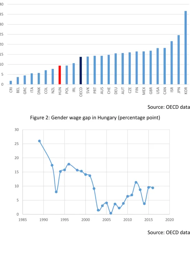
According to the OECD database the gender wage gap has a decreasing trend in Hungary, and it is one of the smallest within the OECD countries. Figures about the trend in Hungary and the size of the gender wage gap in 2016 in OECD can be found in the Appendix. In connection with the gender wage gap OECD (2018) emphasizes the consequences of childbirth on female carrier paths. Women tend to stay at home with children resulting in less working experience,
3
and missing carrier opportunities, that lead to lower income.1 Furthermore, a job can have such non-financial features as unstressed workplace, less competitiveness or more flexible hours which may accord better with the needs of parenting. However, these features can produce self-sorting in the labor market of a kind that women end up in working in lower paid jobs than men. Thus, the distribution of women and men are not equal across occupations.
For example, Blau-Kahn (2000) and Hegewisch-Hartmann (2014) found this kind of segregation decreased till the 2000s, but still exists in the USA.
Lovász (2013) argued that the non-financial features are present more distinctively in the public than in the private sector in Hungary, and this can be the cause of why working in the public sector is so attractive for women. Unfortunately, these non-financial features are less easily measured. Also, there is a significant difference between private and public sector wages because wages are determined by political decisions in public sector while in private sector wage setting is affected by market conditions. (Gregory–Borland (1999)) “Moreover, anti-discrimination legislation may be more aggressively enforced in the public sector and there is evidence that occupational integration has been more rapid in public-sector employment.” (Barron-Cobb-Clark (2008), pp. 2) Thus the wage gap is higher in the private sector, as it is documented by Greene-Hoffnar (1996) in the USA, Barron and Cobb-Clark (2008) on Australian data, Chatterji et al. (2007) in Britain, Cheng (2005) in Canada, and Lovász (2013) in Hungary. Because of these differences between sectors we focus on only the private sector in this study.
In the literature the most frequently applied method for analyzing earning differences consists in regressing the female-male income ratio on individual and job characteristics, and interpreting the unexplained part as a measure of discrimination. Beside individual and job characteristics some researchers have controlled for occupation as well. Kee (2005) and Barron and Cobb-Clark (2008) found that the Australian gender wage gap increased when they used occupation and industry variables. Chatterji et al. (2007) had similar results in Britain. In contrast Altonji and Blank (1999) in the USA, and Cheng (2005) on Canadian data, argued that controlling for occupation decreased the unexplained part of the regression. So, results from the literature are contradictory. Here, we focus on gender wage differences in occupations separately, and use a different method, namely the Random Forest algorithm that we describe in the next section.
3 The Random Forest Regression algorithm
We give a short description of Regression Trees, and Random Forests to build intuition.
Technical and detailed descriptions are available in the original publication of Breitman et al.
(1984), and for a modern survey see Loh (2014).
When growing a regression tree, one starts with the whole sample. The sum of squared deviations from the sample mean are calculated, as the sample mean is considered the first temporary prediction for the full sample. Then one considers each explanatory variable (feature), and calculates by how much the total sum of squared deviations would be reduced
1 For a detailed analysis about the connection of gender wage gap and motherhood in Hungary, see Cukrowska- Lovász (2014).
4
if the full sample were split in two, based on the variable in question, and one would consider the simple average for both subsamples as the prediction over that subsample. (In fact, tree- building methods may differ in how explanatory variables are selected for consideration.) If a variable has many possible values then there are many splits, and one must choose the one with the highest reduction in the sum of squared deviations. After considering each variable in turn, the one with the highest SSE reduction is selected, and the corresponding split of the sample is performed. Graphically this is equivalent to forming two nodes in a tree whose parent node is the root. In other words, the result is a partition of the input space. Later on, one progresses by determining new disjoint subsamples, where for each subsample the average is regarded as the prediction over that subsample. SSE reduction can be viewed alternatively as purifying: the new nodes are purer than the root node, in the sense that the observations belonging to them are on average closer to each other. Tree-building is a recursive process. In the next step each descendant node is considered likewise, and new nodes are added by the same procedure. In practice researchers apply some stopping criterion by limiting, for instance. the number of objects in end nodes.
A Random Forest Regression is constructed from a collection of many Regression Trees, indeed the number of trees is a parameter set by the researcher. The prediction (estimate) a Random Forest regression gives is the average prediction provided by the trees. Each tree is built from a bootstrap sample, which is an important point concerning variable importance measures. The specificity of tree-growing in Random Forests is that at each node only a random subset of explanatory variables are considered for a split. (The cardinality of the subset is another parameter of the algorithm.)
The main advantage of Random Forests is that the random and restricted choice of splitting variables achieves de-correlation among the many trees, while unbiasedness is not jeopardized. (Hastie et al. (2009)) Varian (2015) proposed Random Forests for econometricians by citing Howard and Bowles (2012) who asserted that Random Forests were the most successful general-purpose predictive algorithm. Wager and Athey (2015) argue that Random Forest regression is similar to other traditional non-parametric regression methods (e.g. k-nearest-neighbor algorithms), as it gives some weighted average of “nearby” points as prediction. However, both the weights and the “nearbyness” are determined in a data-driven way. All in all, with the presence of significant non-linearities and with a relative abundance of explanatory variables Random Forest seems to be a successful and well-attested predictive methodology.
Though a successful method for prediction Random Forests have a problem: the results are not easily interpretable variable-wise. The demand for assessing the separate role of variables (their individual explanatory power) led to the proposal of several variable importance measures. In this article we will use the permutation based MSE reduction indicator, that works like this. As trees are grown from bootstrap samples each tree has a number of out-of- the-bag (OOB) observations, i.e. those data points that are not included in the sample for that particular tree. One can then calculate the prediction MSE for OOB data for each tree. Now the idea is that if a variable is unimportant it does not matter whether the predictions are generated with the help of their true values, or are calculated from a random permutation of the true data. (The permutation shuffles only the values of the variable in question.) Then one can calculate the difference between the true and the permuted SSE, which must be small if the variable is unimportant. By averaging all such differences over all trees one obtains a
5
measure of variable importance. (Its properties have been analyzed by simulation by Grömping (2009).) This measure is obviously ad hoc. We will use it in two ways: either ordinally (determining the importance ranking of variables) and by calculating relative importance shares for each variable.
4 Data and methodology
The dataset used in this study is the Hungarian Wage Survey Data, hosted by the National Employment Office. It provides yearly information on workers’ year of birth, gender, occupation, earnings (disaggregated into regular pay and irregular bonuses), type of contract, and whether the worker was hired recently. It also contains information about the employer (sector, region, settlement type, size of employment). The data are recorded for May of each year. The sampling procedure of corporate employees is based on firm size.
The Hungarian Occupational Classification System (FEOR) roughly corresponds to ISCO (International Standard Classification of Occupations).
Table 1
List of variables
Name Unit
Gender 0=Female, 1=Male
Age Years
Tenure Months (at current employer)
Education 9 levels
(levels 8 and 9 are College and University) New entrant dummy 0=no, 1=yes
Share of foreign property 4 levels Share of state property 4 levels
Firm size Number of employees
Settlement Budapest (capital city)
Town Village
Region 7 categories
Sector 20 categories
Collective agreement dummy 0: no, 1: yes Share of white collar employees percentage
For our calculations we used the randomForest R package. The Random Forest algorithm requires the setting of several parameters. In particular, our forests contained 500 trees each.
(In fact, usually the output becomes relatively stable with 100 trees, but the more trees we have the more stable or safer our results are, without important additional costs.) Controlling for the growth of individual trees we set the minimum node-size parameter at 5, which is the
6
usual choice for random forest regressions, and we did not limit the maximum number of nodes. At every node the number of randomly selected variables was 5, roughly in accordance with the default (total number of variables divided by 3).
For all years between 2011 and 2015 we ran random forest regressions for each job category, and computed OOB based variable importance measures as defined above. We consider gender as an important variable if at least in two years out of five the variable importance is above 5 percent. We also determined whether the rank of gender was among the three most important out of the 13 explanatory variables. As we are interested in finding out whether the random forest methodology add new information to what could be achieved by a traditional linear regression model, linear regressions were also run with the same variables for each year, and determined whether gender is significant at the 5 percent level. Moreover, we calculated for every linear regression the variable importance measure proposed by Grömping (2009). This measure is intended to capture the average decrease in SSE attributable to each explanatory variable in a linear regression model. As in any regression the variable specific reduction depends on the rank order of the variable in question, for all possible permutations of variables the SSE reductions are computed for each variable, and then averaged. (We used the Relaimpo R package for the computations.)
5 Results
First, we overview results grouped by main occupational groups. Tables 2-10 show statistics for three-digit occupational categories: whether gender is important in the Random Forest, and in linear regressions, whether gender is significant and positive in linear regression, the male ratio in the sample, and the average educational level.
Group 1 Managers (5 categories)
There are five categories of managers in the three-digit classification, and gender is not an important variable in any of them according to the Random Forest regressions. In all of these categories education, the ratio of foreign ownership and firm size are the most important variables, while in all categories the regression coefficients of gender are positive and significant. Three of these categories are male dominated, (133) is, however, one where females and males are equally present. Only here (133) gender is important in linear regressions.
Table 2
Results of Random Forest and OLS regression in Managers FEOR code maleratio Average
education RF
importance OLS
significance OLS
importance
121 80 7.1 N + N
131 90 7 N + N
132 74 7.4 N + N
133 46 6.4 N + Y
141 56 7.8 N + N
Source: Hungarian Wage Survey Data, own calculation
7
Group 2 Professionals (14 categories)
Of all groups Group 2 has the highest average level of education, it is more homogenous in that respect than Group 1. By the RF importance measure gender is nowhere important in this group. Here firm size, foreign ownership and the share of white collar workers are in general the most important variables. On the other hand, in five job categories gender is important by the LR importance criterion, whereas in almost all of them the regression coefficient is significant.
Table 3
Results of Random Forest and OLS regression in Professionals FEOR code Male ratio Average
education RF
importance OLS
significance OLS
importance
211 86 8.5 N + N
212 94 8.6 N + N
213 83 8.5 N + Y
214 89 8.4 N + N
215 85 7.4 N * N
216 57 8.8 N + N
221 35 8.9 N 0 N
251 41 8 N + Y
252 43 7.9 N + N
253 53 7.9 N + N
261 44 8,8 N 0 N
262 48 8.5 N + Y
271 58 7.6 N + Y
291 53 8.3 N + Y
Source: Hungarian Wage Survey Data, own calculation
Group 3 Technicians and Associate Professionals (18 categories)
Now we descend on the education ladder, and we can find an occupation where gender is important by the RF criterion (313). Again the most important variables are size, foreign ownership and the white collar worker ratio. There are 8 categories of 18 with LR importance, but the gender parameter significance shows a more mixed picture.
8 Table 4
Results of Random Forest and OLS regression in Technicians and Associate Professionals FEOR code Male
ratio
Average education
RF
importance OLS
significance OLS
importance
311 73 6.1 N + Y
312 96 5.8 N 0 N
313 64 5.8 Y + Y
314 70 6.1 N + N
315 65 5.4 N + Y
316 75 6.4 N + Y
319 77 6.2 N + Y
321 88 6.3 N + N
322 41 6.2 N 0 N
331 6 5.2 N 0 N
332 5 5.6 N + Y
333 41 5.6 N 0 N
361 20 6.3 N + Y
362 51 6.2 N + N
363 36 6.4 N + N
364 12 6.7 N 0 N
371 59 6.3 N + Y
391 35 6.3 N + Y
Source: Hungarian Wage Survey Data, own calculation
Group 4 Clerical Support Workers (6 categories)
Further slight fall in average education. The majority of these occupations is female dominated, there is only one category where the male ratio is higher than 50 percent. No gender importance could be found in either sense, and only in two cases are the regression parameters significant.
Table 5
Results of Random Forest and OLS regression in Clerical Support Workers FEOR code Male
ratio
Average education
RF
importance OLS
significance OLS
importance
411 10 6.0 N 0 N
412 12 6.4 N 0 N
413 51 5.6 N 0 N
419 25 6.1 N + N
421 13 5.6 N 0 N
422 27 6.3 N + N
Source: Hungarian Wage Survey Data, own calculation
9
Group 5 Services and Sales Workers (7 categories)
From here on the occupations require only low education levels. Otherwise the results are similar to the previous ones. Gender is not important by the RF criterion, and only in two cases by the LR criterion, but regression coefficients tend to be significant.
Table 6
Results of Random Forest and OLS regression in Services and Sales Workers FEOR code Male ratio Average
education RF
importance OLS
significance OLS
importance
511 25 4.5 N + Y
512 66 4.5 N + N
513 58 4.4 N + Y
523 69 4.8 N 0 N
524 64 4.6 N 0 Y
525 93 4.4 N 0 N
529 69 4.5 N + N
Source: Hungarian Wage Survey Data, own calculation
Group 6 Skilled Agricultural, Forestry and Fishery Workers (2 categories)
In these two male-dominated occupations gender is not important by RF, but important by the LR criterion, and in both cases the regression coefficients are significant.
Table 7
Results of Random Forest and OLS regression in Skilled Agricultural, Forestry and Fishery Workers
FEOR code Male ratio Average education
RF
importance OLS
significance OLS
importance
611 65 4.1 N + Y
612 79 3.3 N + Y
Source: Hungarian Wage Survey Data, own calculation
Group 7 Craft and Related Trades Workers (7 categories)
Here appear two occupations where gender is an important variable by the RF criterion, and in five it is important by the LR, while significance prevail in all categories. The most important variable appears to be firm size, but foreign ownership loses its importance. There are also two categories (741,742) where gender enters among the most important three variables.
Both of these occupations are relatively male dominated, but not overwhelmingly.
10 Table 8
Results of Random Forest and OLS regression in Craft and Related Trades Workers FEOR code Male ratio Average
education RF
importance OLS
significance OLS
importance
711 69 3.8 N + N
721 16 3.9 N + Y
722 92 4.0 N + N
723 72 4.5 Y + Y
734 93 4.7 N + Y
741 63 3.7 Y + Y
742 79 4.5 Y + Y
791 74 4.5 N + Y
Source: Hungarian Wage Survey Data, own calculation
Group 8 Plant and Machine Operators and Assemblers (8 categories)
In 5 categories gender is important according to the RF measure, and in each one by the LR criterion. Needless to say the regression coefficients are always significant. Some of these groups are male dominated but the same results apply to those jobs where women are in the majority. In categories 813 and 819 gender is among the most important three variables.
Otherwise firm size is generally the most important, and foreign ownership does not belong to the most important variables.
Table 9
Results of Random Forest and OLS regression in Plant and Machine Operators and Assemblers FEOR code Male ratio Average
education RF
importance OLS
significance OLS
importance
811 75 3.9 Y + Y
812 35 3.5 Y + Y
813 71 4.2 Y + Y
814 80 3.5 N + Y
815 86 3.9 N + Y
819 48 3.9 Y + Y
821 37 3.9 Y + Y
832 86 4.2 N + Y
Source: Hungarian Wage Survey Data, own calculation
Group 9 Elementary Occupations (6 categories)
These occupations require the lowest level of education. In each category the regression coefficient is significant, gender is important by the LR criterion, and definitely important in three categories by the RF criterion.
11 Table 10
Results of Random Forest and OLS regression in Elementary Occupations FEOR code Male ratio Average
education RF
importance OLS
significance OLS
importance
911 26 3.0 Y + Y
921 65 3.0 N + Y
922 66 3.4 Y + Y
923 56 3.3 Y + Y
931 59 3.1 N + Y
933 76 3.1 N + Y
Source: Hungarian Wage Survey Data, own calculation
6 Conclusions
Our LR importance criterion is obviously stronger than simple significance. However, the RF criterion is even more selective. It seems that intra-occupationally gender is definitely important for jobs where the educational requirements are low, largely independently of the share of males in the given job. One could even say that there is a tendency towards less and less gender importance as we climb upwards on the educational scale.
Hungary is a country where the gender pay gap is below the OECD average. It is also a country where the premium on education is one of the highest. Our results suggest that the vanishing of the overall pay-gap is partly due to the fact that in higher skilled jobs the occupational pay- gap is not large, whereas it obscures the fact that in lower-paid unskilled jobs it is still very much extant.
7 References
Altonji, J. G.–Blank, R. M. (1999): Race and Gender in the Labor Market. In: Ashenfelter, O.–
Card, D. (edit.): Handbook of Labor Economics. Elsevier, Amsterdam, Vol. 3, pp. 3144–3259 Barron, Juan D–Cobb-Clark, Deborah A. (2008): Occupational Segregation and the Gender Wage Gap in Private- and Public-Sector Employment: A Distributional Analysis, IZA Discussion Papers, No. 3562.
Blau, Francine D.–Lawrence, M. Kahn (2000): Gender differences in pay. Journal of Economic perspectives, Vol. 14, pp. 475-99
Breiman, L.–Friedman, J.–Stone, C. J.–Olshen, R. A. (1984): Classification and regression trees.
CRC Press.
Chatterji, Monojit–Mumford, Karen–Smith, Peter N. (2007): The public-private sector gender wage differential in Britain: evidence from matched employee-workplace data. Applied Economics, Vol. 43, No. 26, pp. 3819-3833
Cheng, X. (2005) The Gender Wage Gap in the public and Private Sectors in Canada, thesis, University of Saskatchewan
Cukrowska, Ewa–Lovász, Anna (2014): Are children driving the gender wage gap? Comparative evidence from Poland and Hungary. Institute of Economics, Centre for Economic and Regional
12
Studies, Hungarian Academy of Sciences Department of Human Resources, Corvinus University of Budapest, Budapest Working Papers on the Labour Market, Vol. 4
Goldin, Claudia (2014): A grand gender convergence: Its last chapter. American Economic Review, Vol. 104, No. 4, pp. 1091-1119
Greene, Michael–Hoffnar, Emily (1996): Gender discrimination in the public and private sectors: A sample selectivity approach, Journal of Socio-Economics, Vol. 25, No. 1, pp. 105-114 Gregory, Robert G.–Borland, Jeff (1999): Recent developments in public sector labor markets.
In: Ashenfelter, O.–Card, D. (edit.): Handbook of Labor Economics, Vol. 3, Part C, pp. 3573- 3630
Grömping, Ulrike (2009): Variable importance assessment in regression: linear regression versus random forest. The American Statistician, Vol. 63. No. 4, pp. 308-319.
Hastie, Trevor – Tibshirani, Robert – Friedman, Jerome [2009]: The Elements of Statistical Learning. Data Mining, Inference, and Prediction. Springer-Verlag,New York.
Hegewisch, Ariane–Hartmann, Heidi (2014): Occupational segregation and the gender wage gap: a job half done. Institute for Women's Policy Research, prepared for the Women's Bureau, U.S. Department of Labor.
Howard, J., & Bowles, M. (2012). The two most important algorithms in predictive modeling today. In Strata Conference: Santa Clara.
Kee, Hiau Joo (2005): Glass ceiling or sticky floor? Exploring the Australian gender pay gap using quantile regression and counterfactual decomposition methods. CEPR Discussion Papers 487, Centre for Economic Policy Research, Research School of Economics, Australian National University
Loh, Wei Yin (2014): Fifty years of classification and regression trees. International Statistical Review, Vol. 82, Issue 3, pp. 329--348
Lovász, Anna (2013): Jobbak a nők esélyei a közszférában? A nők és a férfiak bérei közötti különbség és a foglalkozási szegregáció vizsgálata a köz- és magánszférában. Közgazdasági Szemle, Vol. 60, July-August, pp. 814-836.
OECD (2018): OECD Employment outlook. OECD Publishing, Paris OECD database: Gender wage gap
Link: https://data.oecd.org/earnwage/gender-wage-gap.htm#indicator-chart Downloaded: 4st December 2018
Varian, Hal R (2014): Big data: New tricks for econometrics. Journal of Economic Perspectives, Vol. 28, No. 2, pp. 3-28.
Wager, S., & Athey, S. (2017). Estimation and inference of heterogeneous treatment effects using random forests. Journal of the American Statistical Association.
13
Appendix
Figure 1: Gender wage gap in 2016 in OECD countries (percentage point)2
Source: OECD database Figure 2: Gender wage gap in Hungary (percentage point)
Source: OECD database
2 „The gender wage gap is defined as the difference between median earnings of men and women relative to median earnings of men.” (OECD)
0 5 10 15 20 25 30 35 40
CRI BEL GRC ITA DNK COL NZL HUN POL IRL OECD SVK PRT AUS CHE DEU AUT CZE FIN MEX GBR USA CAN ISR JPN KOR
0 5 10 15 20 25 30
1985 1990 1995 2000 2005 2010 2015 2020