Efficient evaluation of the geometrical first derivatives of three-center Coulomb integrals

(1)

Efficient evaluation of the geometrical first derivatives of three-center Coulomb integrals

Gyula Samu, and Mihály Kállay

Citation: The Journal of Chemical Physics 149, 124101 (2018); doi: 10.1063/1.5049529 View online: https://doi.org/10.1063/1.5049529

View Table of Contents: http://aip.scitation.org/toc/jcp/149/12 Published by the American Institute of Physics

(2)

Efficient evaluation of the geometrical first derivatives of three-center Coulomb integrals

Gyula Samuâ)and Mihály Kállay^b)

MTA-BME Lend¨ulet Quantum Chemistry Research Group, Department of Physical Chemistry and Materials Science, Budapest University of Technology and Economics, P.O. Box 91, H-1521 Budapest, Hungary (Received 23 July 2018; accepted 7 September 2018; published online 24 September 2018)

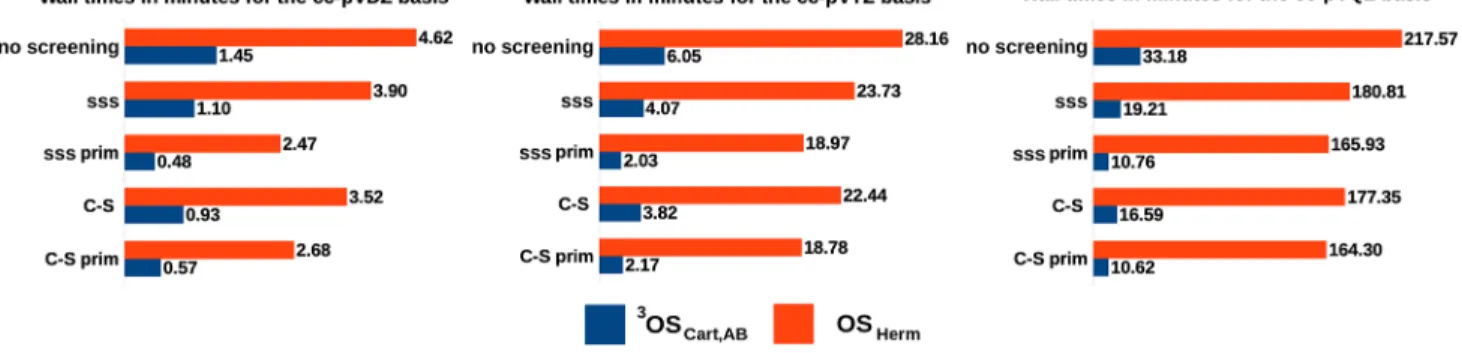
The calculation of the geometrical derivatives of three-center electron repulsion integrals (ERIs) over contracted spherical harmonic Gaussians has been optimized. We compared various methods based on the Obara–Saika, McMurchie–Davidson, Gill–Head-Gordon–Pople, and Rys polynomial algorithms using Cartesian, Hermite, and mixed Gaussian integrals for each scheme. The latter ERIs contain both Hermite and Cartesian Gaussians, and they combine the advantageous properties of both types of basis functions. Furthermore, prescreening of the ERI derivatives is discussed, and an efficient approximation of the Cauchy–Schwarz bound for first derivatives is presented. Based on the estimated operation counts, the most promising schemes were implemented by automated code generation, and their relative performances were evaluated. We analyzed the benefits of computing all of the derivatives of a shell triplet simultaneously compared to calculating them just for one degree of freedom at a time, and it was found that the former scheme offers a speedup close to an order of magnitude with a triple-zeta quality basis when appropriate prescreening is applied. In these cases, the Obara–Saika method with Cartesian Gaussians proved to be the best approach, but when derivatives for one degree of freedom are required at a time the mixed Gaussian Obara–Saika and Gill–Head- Gordon–Pople algorithms are predicted to be the best performing ones.Published by AIP Publishing.

https://doi.org/10.1063/1.5049529

I. INTRODUCTION

Analytical derivative methods are essential tools of quantum chemistry^1,2since many of the most important molecular properties are related to energy derivatives. The geometrical gradient of the energy is necessary to find equilibrium structures of chemical systems, which makes it especially of interest. The speed of the evaluation of electron repulsion integral (ERI) derivatives is an important factor in the efficiency of such gradient calculations.³

When Cartesian Gaussian basis functions are applied, the ERI derivatives can be computed in a straightforward man- ner invoking the differentiation rule of the Gaussians after the evaluation of the ERIs. More elaborate techniques were also investigated in the literature that proved useful in accelerating four-center ERI derivative calculations. With the Rys polynomial method,^4–7 where ERIs are calculated as the weighted sum of two-dimensional integral products, one can differentiate these intermediates and calculate the ERI derivatives directly.^8,9 Using the McMurchie–Davidson (MD) expansion,¹⁰the cost of the derivative integral computation can be reduced by differentiating the Hermite integrals and the corresponding expansion coefficients with respect to variables related to nuclear coordinates and then, after an assembly, transforming these derivatives into the desired quantities.¹¹ The Gill–Head-Gordon–Pople (GHP) algorithm,^12,13 which

a)Electronic mail: gysamu@mail.bme.hu

b)Electronic mail: kallay@mail.bme.hu

transforms the Hermite integrals of the MD scheme into ERIs over Cartesian overlap distributions using contracted level recursions, can be used to compute derivatives as well.^14,15The accompanying coordinate expansion and transferred recurrence relation method,¹⁶efficient for the computation of ERIs with heavily contracted basis sets, was also extended to serve derivative calculation purposes.¹⁷It was shown in Ref.18that Hermite Gaussians are also applicable to ERI and ERI derivative calculations when the angular parts of the basis functions are spherical harmonics, and the Obara–Saika¹⁹ (OS) recurrences for Hermite ERIs were also presented. The use of Hermite Gaussians offers the advantage of a more simple calculation of derivatives from the ERIs compared to Carte- sian Gaussians, although the horizontal recurrence relation²⁰ (HRR) involves four terms instead of the original two. The translational and rotational invariance of ERIs and their application to derivative evaluations were also investigated by several authors.^21–27

Density fitting (DF) is an established procedure to efficiently and accurately approximate the four-center ERIs required by most quantum chemical methods. If the Coulomb metric is applied for DF,^28–32then three- and two-center ERI derivatives are necessary to evaluate the derivative of the energy. Here the efficiency is determined by the speed of the three-center ERI derivative calculation, for which, in princi- ple, all of the above mentioned methods can be adapted. While this has not been done so far, several techniques have been developed for the evaluation of three-center ERIs, which are also useful in accelerating the computation of their derivatives.

0021-9606/2018/149(12)/124101/20/$30.00 149, 124101-1 Published by AIP Publishing.

(3)

Ahlrichs showed³³ that the OS method can be considerably simplified if the fitting functions have spherical harmonic angular parts. In our recent work, we proved³⁴that the computation of the two-dimensional integrals of the Rys method also becomes simpler in this case. The MD and GHP algorithms greatly benefit from the use of spherical harmonic Hermite Gaussians for the ket side of three-center ERIs since the time consuming transformation of Hermite Gaussians into the Cartesian ones can be avoided for the fitting functions.¹⁸ We should also mention the work of K¨oster, who combined the OS, MD, and GHP methods for three-center ERIs³⁵ and developed new recurrence formulas for fitting basis sets con- taining uncontracted Hermite Gaussian functions.³⁶Efficient implementation of three-center ERIs and ERI derivatives,^37–40 as well as options for prescreening these quantities,^41–43has also received attention.

It is worth mentioning that the explicit evaluation of the three-center ERI derivative list is not mandatory for the computation of the derivative of the Coulomb-energy in a direct self-consistent field (SCF) calculation. Utilizing the J-engine scheme and related ideas,^36,44 it is possible to only partially calculate the integral-derivatives and, by reverse operations, transform the density matrix into a form appropriate for the contraction with intermediate differentiated ERIs rather than with those over atomic orbitals (AOs). The approach is especially advantageous for Kohn–Sham SCF gradients, but it can also be beneficial for DF Hartree–Fock or hybrid density functional calculations if the J-engine is applied along with reduced-cost schemes^45–51 for the computation of the Fock-exchange contribution to the gradient. In the latter cases, however, three-center ERI derivatives still have to be computed. In addition, the ideas of the J-engine approach cannot be efficiently utilized for correlated gradient calculations. We also note that, for basis functions with sufficiently small overlap, the exact calculation of ERI derivatives is not necessary.

Here significant speedups can be achieved by the application of approximations based on multipole or asymptotic expan- sions.^52–54 Still, the evaluation of the near-field ERI derivatives demands considerable computational effort, especially in the case of integrals involving high angular momentum functions.

In this study, our goal is to find the most efficient method for evaluating three-center ERI derivatives using contracted spherical harmonic Gaussians. In Sec.II, we summarize the properties of Cartesian and Hermite Gaussian basis functions and three-center ERI derivatives and discuss the adaptation of the OS, MD, GHP, and Rys schemes for calculating the derivatives for Cartesian and Hermite Gaussian integrals. We give new recurrence relations for each method to evaluate mixed Gaussian ERIs, which contain both Cartesian and Hermite Gaussians. The motivation for using these integrals is to benefit from both the easier derivative calculation with Hermite Gaussians and the less expensive Cartesian recurrences. We note that, to our knowledge, the MD, GHP, and Rys methods have not yet been extended to the case of Hermite Gaussian basis functions, and this has been achieved in the present work.

We explore schemes for evaluating the ERI derivatives sepa- rately for each degree of freedom and also the ones where all of the derivatives are computed at the same time. The latter

approach makes us able to exploit the translational invariance of the integrals and use shared recursion intermediates for the derivative calculations. We also consider different prescreening approaches, introducing an efficient approximation of the Cauchy–Schwarz upper bound for ERI derivatives. SectionIII presents and discusses floating point operation (FLOP) counts for the considered algorithms. In Sec. IV, implementation details are given, and in Sec.V, we compare the runtime performances of the selected schemes, which we implemented by automated tools, as well as the four prescreening approaches described in Sec. II F. We summarize our conclusions in Sec.VI.

II. THEORY

A. Geometrical derivatives of three-center Coulomb integrals

In this work, we investigate the efficient evaluation of the first-order geometrical derivatives of three-center Coulomb integrals over contracted solid harmonic Gaussian functions using integrals over Cartesian and Hermite Gaussians. The Cartesian Gaussians have the form of

G_IJK(r,a,A)=x_A^Iy^J_Az_A^Kexp

−ar_A²

, (1)

and the Hermite Gaussians will be defined as¹⁸ H˜˜I˜JK˜(r,a,A)= ∂^L^˜exp(−ar_A²)

(2a)^L^˜∂A^˜Î_x∂A^J_y^˜∂A^K_z^˜, (2) whererdenotes the position vector of the electron,Ais the position of the center of the function,ais a constant Gaussian exponent, andr_Ais the magnitude of the vectorr_A=r−Awith x_Abeing the x component ofr_A.L=I+J+Kwill be called the angular momentum of the Gaussian, and the vectorL= (I,J, K) will be referred to as its angular momentum vector. A tilde over the angular momentum vector and its components will be used for Hermite Gaussians to distinguish them from the corresponding Cartesian Gaussians. Functions with the same center, exponent, and angular momentum constitute a shell with (L+ 1)(L+ 2)/2 components. The primitive Gaussians are sep- arable in the three Cartesian directions, that is,G_IJK=G_IG_JG_K and ˜H_I_˜_J_˜_K_˜ =H˜_˜_IH˜_J_˜H˜_K_˜, where, for instance,G_I=x_AÎ exp(−ax²_A) and ˜H_I =∂Î^˜exp(−ax_A²)/(2a∂A_x)^˜Î. Cartesian Gaussians obey the recurrence relations

x_AG_I=G_I+1 (3)

and ∂G_I

∂A_x =2aGI+1−IG_I−1, (4) while the corresponding relations for the Hermite Gaussians are

x_AH˜˜I=H˜_˜_I+˜1+ ˜I

2aH˜_˜_I−˜1 (5)

and ∂H˜_I_˜

∂Ax =2aH˜_˜_I+˜1. (6) We will also make use of the

x_B=x_A+X_AB (7)

(4)

equation. In some cases, we will utilize the unscaled Hermite Gaussians, defined as

H¯I¯JK¯(r,a,A)= ∂^L^¯exp(−ar_A²)

∂A^I_x^¯∂A^J_y^¯∂A^K_z^¯ . (8) A shell of differentiated Cartesian Gaussians can be transformed into a differentiated solid harmonic Gaussian shell consisting of 2L+ 1 functions as

∂G_Lm(r,a,A)

∂A_x = X

I+J+K=L

C^Lm_IJK∂G_IJK(r,a,A)

∂A_x , (9) wheremis an integer satisfying−L ≤m ≤L, and theC_IJK^Lm coefficients in Eq.(9)only depend on the angular momentum vector and the value ofLandm.⁵⁵Equation(9)also holds for undifferentiated Cartesian Gaussians. For the transformation of the Hermite Gaussians, the values of the coefficients are the same as in the Cartesian case,¹⁸and the simple differentiation rule, Eq.(6), allows us to perform the differentiation and the

transformation in a single step as

∂G_Lm(r,a,A)

∂A_x = X

˜I+˜J+ ˜K=L˜

C_˜^Lm

IJ˜K˜2aH˜˜I+˜1˜JK˜(r,a,A), (10) whereC_˜^Lm

I˜JK˜ =C_IJK^Lm. We obtain contracted Gaussians (and differentiated contracted Gaussians analogously) by combining the corresponding elements of shells with different exponents as

χ_ALm(r,A)=X

a

G_Lm(r,a,A)daχA, (11) where the contraction coefficientsd_aχ_A also include the norm of the solid harmonic Gaussian function and are the same for a given shell. The solid harmonic transformation and the contraction of primitives are interchangeable operations even if we use Eq.(10)since in practice the multiplication with 2ais performed on earlier stages of the calculation.

Three-center ERIs over primitive Cartesian Gaussian functions are defined as

(LaLb|Lc)= G_I_a_J_a_K_a(r₁,a,A)GIbJbKb(r₁,b,B)GIcJcKc(r₂,c,C)

|r₁−r₂| dr1dr2, (12)

whereLa= (Ia,J_a,K_a) stands for the angular momentum vector, andL_a=I_a+J_a+K_ais the angular momentum of the function with exponenta. Likewise, the ERIs over primitive Hermite Gaussian functions are given as

( ˜LaL˜b|L˜c)= H˜_˜_I

aJ˜aK˜a(r1,a,A) ˜H_˜_I

bJ˜bK˜b(r1,b,B) ˜H_˜_I

cJ˜cK˜c(r2,c,C)

|r₁−r₂| dr1dr2. (13)

The term class will be used to refer to primitive or solid harmonic integrals with the same angular momenta, centers, and exponents; e.g., the primitive class (11|1) contains 27 primitive integrals. For contracted integrals, a class will mean a group of ERIs over the same contracted functions and with the same angular momenta and centers. A shell triplet will refer to all the integrals belonging to the same centers and angular momenta.

The primitive integral where the total angular momentum is zero is of central importance for the evaluation of ERIs. For both types of basis functions, the value of this integral is given explicitly as³³

(00|0)≡(00|0)⁽⁰⁾=θ_pcκ_abF₀(αR²_PC), (14) with

κ_ab=exp(−µR²_AB), θ_pc = 2π^5/2 pc√

p+c, µ= ab

a+b, P=aA+bB

p , R_AB=A−B, R_PC=P−C,

p=a+b, α= pc

p+c andF_nbeing the Boys function of ordern, defined as

F_n(x)= ₁

0

t²ⁿexp(−xt²)dt. (15)

Integrals (00|0)⁽ⁿ⁾calculated similar to Eq.(14)with the order of the Boys function not necessarily being zero serve as the starting values for the OS,¹⁹ MD,¹⁰ and GHP¹² schemes for the evaluation of the integrals of Eqs.(12)and(13)and their derivatives.

Generally, differentiation of the integrals defined by Eqs.(12)and(13)results in a linear combination of integrals over differentiated basis functions given by Eqs.(4)and(6)as

∂(L_aLb|Lc)

∂A_x =∂L_a

∂A_xL_b|Lc

+ La

∂L_b

∂A_x|Lc

+

LaL_b|∂L_c

∂A_x . (16) In the following, we will utilize the translational invariance of the integrals,

∂L_a

∂A_xLb|Lc

+ La

∂L_b

∂B_x|Lc

+

LaLb|∂L_c

∂C_x

=0. (17) First of all, it trivially follows that Eq.(16)evaluates to zero if the three functions are located on the same center. Rearranging Eq.(17), we get

∂L_a

∂A_xL_b|Lc

+ La

∂L_b

∂B_x|Lc

=−

LaL_b|∂L_c

∂C_x

, (18) from which two further things are apparent. First, if two of the three centers coincide, differentiating with respect to the coordinates of this center does not require the evaluation of the sum in Eq.(16), but rather we can differentiate the third function and take the negative of the result. This does not

(5)

necessarily reduce the operation count since performing the differentiation for this second center can be more expensive than to do so for the functions centered on the first one. How- ever, for medium-sized and larger systems, such integrals are much less numerous than the ones with three distinct centers.

For such shell triplets with coinciding centers, Eq.(18)only makes an optimized code-generated implementation simpler since one does need to have separate subroutines to treat these cases. Second and more importantly, if we wish to produce the derivatives for the shell triplets with respect to all three centers, it is sufficient to perform the calculations only for two of the centers for a given shell triplet, and the derivatives for the third (most expensive) one can be constructed by using Eq. (18). The classes required for these two derivatives can be built up in the same recursive process, reducing the redun- dancy of the calculation. However, proceeding in such a way is not always the preferred choice. For example, producing derivatives with respect to a couple of degrees of freedom at a time may be advantageous for a coarse-grained parallelization scheme where the derivatives with respect to the coordinates of a center are evaluated on a separate node. The similar holds when the solution of response equations is necessary for each degree of freedom, as is the case for the calculation of second derivatives, and we wish to avoid the storage and sorting of the integral-derivatives. For these reasons, we will investigate both approaches.

Utilizing Eq. (18), we only need to explicitly calculate 6 of the 9 derivatives of a three-center ERI. When Carte- sian Gaussians are used, the classes ([La + 1_x]Lb|Lc), ([La

− 1_x]L_b|L_c), (L_a[L_b + 1_x]|L_c), and (L_a[L_b − 1_x]|L_c), for example, have to be evaluated to construct the necessary derivatives. Kahn has shown²⁴that, from the rotational invariance of the integrals, it is possible to recover all of the derivatives of an (L_aL_b|L_c) integral by just computing, for example,

∂(L_aLb|Lc)/∂A_x,∂(L_aLb|Lc)/∂A_y,∂(L_aLb|Lc)/∂B_z, and three other auxiliary integrals which are linear combinations of the ERIs in the (LaLb|Lc) class. The remaining derivatives can be calculated by solving three simultaneous linear equations, optionally at the contracted level. The possible advantage is that not all components of the classes with increased angular momenta have to be evaluated. The approach, however, has drawbacks. It is required to compute the extra class (L_aL_b|L_c).

When the HRR is applied, as is often the case, these ERIs appear as intermediates for (L_a[L_b + 1_x]|L_c). However, this fact cannot be exploited if the buildup of the final angular momenta takes place at the contracted level since according to Eq. (4) the class with incremented L_b will be scaled by 2b, meaning that the class required for the auxiliary integrals has to be computed by a separate recursion. Furthermore, none of the functions of the (L_aL_b|L_c) ERIs can be transformed into the spherical harmonic Gaussian basis until the auxiliary integrals have been formed, while performing these operations on earlier intermediates is known⁷ to enhance the speed of the calculation. This also hinders the exploitation of (LaLb|Lc) as an intermediate of another class. The for- mation of the auxiliary integrals is also relatively expensive, each requiring five additions and six multiplications. The solution of the system of linear equations is also considerably more expensive than the application of Eq.(18). Finally, the

advantage of not evaluating every component of the more expensive classes becomes less significant with the increase of the angular momenta. For example, when we wish to compute every∂(LaLb|Lc)/∂Bz, we need the same number of components from the (La[Lb+1x]|Lc) class as the number of ERIs in (LaLb|Lc), with the ratio of the number of the components in the two classes getting smaller with increasingLb. Because of these considerations, we only deal with the invariance property defined by Eq.(17)in this work.

In the following,L_awill denote the final angular momentum we wish to build up on the function with exponenta.l_a will be used to represent the angular momenta of intermediate classes, that is, classes that are required by the recursions or other transformations to create the final angular momentum. The notation will be similar for the other two functions.

The index ranges for the intermediates reported in this paper were determined on the basis of a method outlined in the supplementary material. Even though the presentation sug- gests that the lower limits of the ranges can take negative values, for brevity, we will not use the notation max(0,l) for these cases but assume that the angular momenta are greater than or equal to zero. The notation for the various investigated methods will display the basic algorithm, the applied basis function, the center the coordinates of which we differentiate with respect to, and an additional index if we inspect different approaches for a given problem. For example, GHPCart,A2will denote the GHP-based scheme where we use Cartesian Gaus- sians and differentiate with respect toA, while the approach to which “2” refers will be explained later. We will omit the indices when we talk about all the possible values for those indices, e.g., OSCart means all the discussed methods within the OS scheme that apply Cartesian Gaussians. We will use an upper left index “3” to denote schemes where all the derivatives of the shell triplets are produced by a common recursion.

For example,³OSCart,ABrefers to the OS-based scheme using Cartesian Gaussians where we simultaneously evaluate the derivatives with respect toAandBby recursion and calculate theCderivatives via Eq.(18).

B. Obara–Saika recursion

The OS scheme utilizes recurrence relations for auxiliary intermediate integrals defined as

(LaLb|Lc)⁽ⁿ⁾= 2 π^1/2

∞ 0

G_I_a_J_a_K_a(r1,a,A)

×G_I_b_J_b_K_b(r1,b,B)GIcJcKc(r2,c,C)

×exp(−|r₁−r₂|²u²) u² α+u²

n

dr1dr2du (19) to construct the true ERIs with n= 0 and with the required angular momenta for the calculation of the differentiated integrals. From now on, superscript (n) will be kept only when it is not equal to zero. For the derivation of the equations for four-center ERIs, we refer to the other work.^19,55

An efficient application of the OS method to three-center solid harmonic Gaussian ERIs was developed by Ahlrichs.³³ Our equations will slightly differ from those of Ref.33since it will prove useful to work with the starting integrals

(6)

(00|0)⁽ⁿ⁾≡(0)⁽ⁿ⁾=(−2α)ⁿθ_pcκ_abF_n(αR²_PC). (20) To arrive at the undifferentiated (LaLb|Lc) class, we first apply the vertical recurrence relation (VRR)

([la+1_x]0|0)⁽ⁿ⁾=X_PA(la0|0)⁽ⁿ⁾+ 1

2pX_PC(la0|0)⁽ⁿ⁺¹⁾ + i_a

2p

([la−1x]0|0)⁽ⁿ⁾ + 1

2p([la−1_x]0|0)⁽ⁿ⁺¹⁾

. (21)

Here and from now on,la+1_xmeans that thexcomponent of the angular momentum vectorla has been increased by one.

To reach an (La0|0)⁽ⁿ⁾class, Eq.(21)needs (00|0)^(m)ERIs for n ≤m ≤n+ L_a. Next, the simplified vertical recurrence for the ket function³³

(la0|[lc+1_x])⁽ⁿ⁾=−1

2cX_PC(la0|lc)⁽ⁿ⁺¹⁾

− i_a

4pc([l_a−1_x]0|l_c)⁽ⁿ⁺¹⁾ (22) is applied, which requires (l_a0|0)⁽ⁿ⁾intermediates forL_a−L_c

≤l_a ≤L_a andn=L_c to construct an (L_a0|L_c) class. Finally, the HRR

(la[lb+1_x]|Lc)=([la+1_x]lb|Lc) +X_AB(lalb|Lc) (23) is employed, for which (la0|Lc)-type intermediates forL_a≤l_a

≤L_a +L_b are needed to build (LaLb|Lc) ERIs. We note that thel_a→l_c→l_border of building up the angular momenta is not the only possible one, and the electron transfer relation⁵⁶ can also be applied in the evaluation of the ERIs. In our pre- vious study,³⁴we found that the presented scheme is the most efficient OS-type algorithm for undifferentiated three-center Cartesian ERIs.

The application of this method is straightforward for the derivatives with respect to the coordinates of A and B, where we use Eqs. (20)–(23) to evaluate the required classes for Eq. (4). This slightly modifies the index ranges;

e.g., for ([∂L_a/∂A_x]L_b|L_c), the lower and upper limits that depend onL_adecrease and increase by one, respectively. Equa- tion(22)can, however, not be applied if we wish to evaluate (LaL_b|[∂Lc/∂Cx]). Instead, we shall use the original VRR equation¹⁹reduced to the three-center case,

(la0|[lc+1_x])⁽ⁿ⁾=−1

2cX_PC(la0|lc)⁽ⁿ⁺¹⁾

− i_a

4pc([la−1x]0|lc)⁽ⁿ⁺¹⁾ + i_c

2c

(la0|[lc−1_x])⁽ⁿ⁾ + 1

2c(la0|[lc−1x])⁽ⁿ⁺¹⁾

. (24) For undifferentiated ERIs, the last two terms of Eq.(24)can- cel when we transform Lc to the solid harmonic Gaussian basis.³³Now we are changing to the differentiated solid harmonic Gaussian basis, and from Eqs.(4)and(9), we can see that functions with angular momenta higher and lower thanL_c get transformed by the coefficients belonging toL_c; hence, the cancellation does not take place. The (l_a0|0)⁽ⁿ⁾ERIs required for the calculation of an (L_a0|L_c) class by using Eq.(24)are

those with the mod[Lc, 2]≤n≤L_candL_a−mod[Lc, 2]−2d(n

−mod[Lc, 2])/2c ≤l_a ≤L_aindex ranges, wheredxcdenotes the integer part ofx.

The OS method can be developed for ERIs over Hermite Gaussians as well.¹⁸The bra side VRR is very similar to its Cartesian counterpart, having the form of

([˜la+ ˜1_x]0|0)⁽ⁿ⁾=X_PA(˜la0|0)⁽ⁿ⁾+ 1

2pX_PC(˜la0|0)⁽ⁿ⁺¹⁾ + ˜i_a

2p −b

a([˜la−1˜_x]0|0)⁽ⁿ⁾ + 1

2p([˜la−1˜_x]0|0)⁽ⁿ⁺¹⁾

. (25)

The VRR for the ket function is the same as Eq.(22). The HRR for the Hermite ERIs,

(˜la[˜lb+ ˜1_x]|L˜c)=([˜la+ ˜1_x]˜lb|L˜c) +X_AB(˜la˜lb|L˜c) + ˜i_a

2a([˜la−1˜x]˜lb|L˜c)− ˜i_b

2b(˜la[˜lb−1˜x]|L˜c), (26) can be obtained with the help of Eqs. (5) and (7). The range for the necessary ( ˜la0|L˜c) intermediates for Eq.(26)is L˜_a−L˜_b ≤˜l_a ≤L˜_a+ ˜L_b. The ERIs required forAandBderiva- tives are computed with the above described scheme with modified index limits; e.g., for ([∂L˜_a/∂A_x] ˜L_b|L˜_c), the lower and upper limits that depend on ˜L_a increase by one according to Eq.(6). Note that the multiplication with the double of the exponent appearing in Eq.(6)can be built into Eq.(20) if we calculate a derivative with respect to one center at a time. When we differentiate with respect toC, the necessary ket VRR equation is analogous to Eq.(24); however, the third term is zero. This is because in the corresponding equation for four-center ERIs¹⁸this third term is multiplied by−d/c, wheredis the exponent for the fourth function, andd is zero for three-center integrals. Hence the relation becomes

(˜l_a0|[˜l_c+ ˜1_x])⁽ⁿ⁾=−1

2cX_PC(˜l_a0|˜l_c)⁽ⁿ⁺¹⁾

− ˜i_a

4pc([˜la−1˜_x]0|˜lc)⁽ⁿ⁺¹⁾ + ˜i_c

4c²(˜la0|[˜lc−1˜_x])⁽ⁿ⁺¹⁾, (27) for which we need ( ˜l_a0|0)⁽ⁿ⁾-type ERIs to build an ( ˜L_a0|L˜_c) class for ˜L_c− dL˜_c/2c ≤n≤L˜_cand ˜L_a+ ˜L_c−2n≤˜l_a ≤L˜_a.

We see that both kinds of Gaussian basis functions have advantageous properties. With Hermite Gaussians, the explicit evaluation of the primitive derivatives can be avoided and the recursion for ˜Lcduring the computation of ( ˜LaL˜b|[∂L˜c/∂C_x]) is simpler, while for the Cartesian Gaussians the HRR is cheaper, independent of the exponents, and requires a smaller range of intermediates. For higherL_bvalues, this latter property compensates for the widening of the index ranges due to Eq. (4), while if the differentiated function is of stype, the direct application of Eq.(4)can be avoided similar to the Her- mite case. In the following, we exploit that, for first derivatives, only one of the functions has to be Hermite Gaussian to utilize Eq.(6), and we shall investigate how calculating such mixed

(7)

Gaussian ERIs affects the complexity of the task. The derivation of the following recurrences can be found in Subsection1 of theAppendix.

For theAderivatives, we choose the first and second bra functions to be a Hermite and a Cartesian Gaussian, respectively, and use Eq. (25) for the bra VRR. Since the choice for the function in the ket side is irrelevant now, we apply Eq.(22)to gain the (˜la0|˜lc)-type intermediates. For the ˜la→lb

translation, we need a new HRR,

(˜la[lb+1x]|˜lc)=([˜la+˜1x]lb|˜lc)+XAB(˜lalb|˜lc)+˜i_a

2a([˜la−˜1x]lb|˜lc), (28) which is one term less expensive than Eq.(26). In the case of the derivatives for B, we reverse the type of the three func- tions and use Eqs.(21)and(22)for the (la0|lc) ERIs and then the

(la[˜lb+ ˜1x]|lc)=([la+1x]˜lb|lc)+X_AB(la˜lb|lc)−˜i_b

2b(la[˜lb−1˜x]|lc) (29) HRR is applied, for which the range of the necessary starting intermediates is the same as for Eq. (23). The obvi- ous choice for theCderivatives is to use the (lalb|˜lc) ERIs since this would allow us to employ Eq.(23)for the HRR.

The appropriate recurrence to construct the (la0|˜lc)⁽ⁿ⁾-type integrals is

(la0|[˜lc+ ˜1_x])⁽ⁿ⁾=−1

2cX_PC(la0|˜lc)⁽ⁿ⁺¹⁾

− i_a

4pc([la−1x]0|˜lc)⁽ⁿ⁺¹⁾ + ˜i_c

4c²(l_a0|[˜l_c−1˜_x])⁽ⁿ⁺¹⁾. (30) Equation(30)is analogous to Eq.(27), but since the function on the first center is now a Cartesian Gaussian, we can use Eq. (23)to build up Lb. In addition to the OS methods for Cartesian (OSCart) or Hermite (OSHerm) Gaussian ERI derivatives, we will also analyze the new schemes based on these mixed Gaussian ERIs (OSMixed) and conclude that the use of such mixed integrals is often superior to the pure Cartesian and always to the pure Hermite algorithms. For the case when the derivatives of all three centers are evaluated at the same time, we will compare the purely Cartesian Gaussian based methods (³OSCart) with³OSHerm,AB,³OSMixed,AC, and³OSMixed,BC. As

we will see, the³OSCart,ABroute is very competitive because of the simple form of Eq.(23). The OS-based algorithms are summarized in TableI.

C. McMurchie–Davidson method

The essence of the MD scheme for undifferentiated ERIs is to recover Gaussian overlap distributions (Cartesian or Hermite) from Hermite Gaussian functions, for which two- center Hermite integrals have to be calculated first. Exploiting the translational invariance of two-center integrals (that is,

−∂/∂Px = ∂/∂Cx), these can be expressed with one-center ERIs as¹⁸

(˜lp|˜lc)⁽ⁿ⁾=(2p)⁻^˜^l^p(2c)⁻^˜^l^c ∂^˜^l^p^+˜^l^c(0)⁽ⁿ⁾

∂P^˜ⁱ_x^p∂P^˜^j_y^p∂P^k_z^˜^p∂C_x^˜ⁱ^c∂C^˜_y^j^c∂C^k_z^˜^c

=(2p)^−˜^l^p(−2c)^−˜^l^c ∂^˜^l^p^+˜^l^c(0)⁽ⁿ⁾

∂P^˜_xⁱ^p^+˜ⁱ^c∂P^˜^j_y^p^+˜^j^c∂P_z^k^˜^p^+˜^k^c

=(2p)⁻^˜^l^p(−2c)⁻^˜^l^c(¯lp+ ¯lc)⁽ⁿ⁾. (31) The one-center quantities on the rightmost side of Eq. (31) can be calculated with the McMurchie–Davidson recurrence¹⁰

(¯l_c+¯l_p+ ¯1_x)⁽ⁿ⁾=X_PC(¯l_c+¯l_p)⁽ⁿ⁺¹⁾+(¯i_p+¯i_c)(¯l_c+¯l_p−1¯_x)⁽ⁿ⁺¹⁾. (32) This relation requires (0)⁽ⁿ⁾ ERIs for dL¯_p/2c+ mod [ ¯L_p, 2]

≤ n ≤ L¯_p to evaluate ( ¯Lp) integrals. From these, one way to recover the three-center integrals is the use of the expression⁵⁵

(L_aL_b|L˜_c)⁽ⁿ⁾=(−2c)^−L^c

Ia+Ib

X

¯ip=0

E_¯^I^a^,I^b

ip Ja+Jb

X

¯jp=0

E_¯^J^a^,J^b

jp

×

Ka+Kb

X

k¯p=0

E^K_¯^a^,K^b

kp (¯lp+ ¯Lc)⁽ⁿ⁾, (33) where it has been utilized that for three-center ERIs over solid harmonic Gaussians we only have to expand the bra side since the Hermite Gaussian in the ket side can be readily transformed into the solid harmonic Gaussian basis. The recursive evaluation of theEexpansion coefficients that transform ¯l_pfunctions intol_al_bproducts is described in Ref.55, and the coefficients to construct ˜l_al˜_bdistributions from ˜l_p functions are presented in Ref.18. It is more efficient³⁴to use recurrences to transform

TABLE I. Serial number of the equations to be applied to calculate the necessary classes in the various OS-based algorithms. Equation(20)is omitted since its use is common to all routes. Separate recursion denotes the schemes where only derivatives with respect to one center are evaluated, while in the common recursion schemes, derivatives for all the centers are calculated at the same time for a shell triplet.

Separate recursion Common recursion

OSCart,Aand OSCart,B (21),(22),(23) ³OSCart,AB (21),(22),(23)

OSCart,C (21),(24),(23) ³OSCart,ACand³OSCart,BC (21),(24),(23)

OSMixed,A (25),(22),(28) ³OSHerm,AB (25),(22),(26)

OSMixed,B (21),(22),(29) ³OSMixed,AC (25),(27),(28)

OSMixed,C (21),(30),(23) ³OSMixed,BC (21),(30),(29)

OSHerm,Aand OSHerm,B (25),(22),(26)

OSHerm,C (25),(27),(26)