Classification and evolution of bifurcation curves for a one-dimensional Neumann–Robin problem

Classification and evolution of bifurcation curves for a one-dimensional Neumann–Robin problem

and its applications

Chi-Chao Tsai

, Shin-Hwa Wang

and Shao-Yuan Huang

1Department of Physics, National Tsing Hua University, Hsinchu 300, Taiwan

2Department of Mathematics, National Tsing Hua University, Hsinchu 300, Taiwan

3Center for General Education, National Formosa University, Yunlin 632, Taiwan

Received 4 March 2018, appeared 8 October 2018 Communicated by Paul Eloe

Abstract. We study the classification and evolution of bifurcation curves of positive solutions for the one-dimensional Neumann–Robin boundary value problem

(u⁰⁰(x) +λf(u(x)) =0, 0<x<1, u⁰(₀) =_{0 and} u⁰(₁) +αu(₁) =_0,

where λ > 0 is a bifurcation parameter,α > 0 is an evolution parameter, and nonlin- earity f satisfies f(0)≥0 and f(u)>0 foru>0. We obtain the multiplicity of positive solutions forα>0 andλ>0. Applications are given.

Keywords: bifurcation, multiplicity, positive solution, Neumann–Robin problem, S- shaped bifurcation curve,⊂-shaped bifurcation curve, time map.

2010 Mathematics Subject Classification: 34B18, 74G35.

1 Introduction

We study the classification and evolution of bifurcation curves of positive solutions for the one-dimensional Neumann–Robin boundary value problem

(u⁰⁰(x) +λf(u(x)) =0, 0< x<1,

u⁰(0) =0 and u⁰(1) +αu(1) =0, (1.1) where λ > 0 is a bifurcation parameter and α > 0 is an evolution parameter. We basically assume that nonlinearity f satisfies the following hypothesis:

(H) f(₀) ≥ 0, f(_u) > _{0 for 0} < _u < _{η, and f} ∈ C[_0,η)∩C²(_0,η)_{, where} η ∈ (_0,∞]_{. In} addition, f(η) = 0 if 0 < η < ∞. (Note that we allow η to be either a finite positive number or infinite.)

BCorresponding author. Email: shwang@math.nthu.edu.tw

Ifα= 0, (1.1) becomes a Neumann boundary value problem. In this case, for allλ>0, it is easy to show thatu(x)≡η<_∞is the unique positive solution. Ifα=∞, (1.1) becomes the Neumann–Dirichlet boundary value problem

(u⁰⁰(x) +λf(u(x)) =0, 0< x<1, u⁰(0) =0 and u(1) =0,

which is equivalent to the Dirichlet boundary value problem (u⁰⁰(x) +λf(u(x)) =0, −1< x<1,

u(−₁) =_{0 and} u(₁) =_0, ^(1.2)

due to symmetry of positive solutionsuon(−1, 1).

We first observe that u is a positive solution of (1.1) with fixed α > 0. Since u⁰⁰(x) =

−λf(u(x))< 0 on(0, 1)and u⁰(0) =0, henceu(x) is strictly concave and strictly decreasing on(0, 1). This implies that

u(0)>u(1). (1.3)

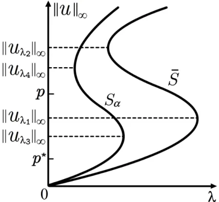
We study the classification and evolution of bifurcation curves of positive solutions of (1.1) defined by

S_α= {(λ,ku_λk_∞):λ>_{0 and}u_λ is a positive solution of (1.1)} (1.4) on the(λ,kuk_∞)-plane when the evolution parameterαvaries from 0⁺ to infinity.

It should be noticed that shapes of bifurcation curves of positive solutions for one- dimensional Dirichlet boundary value problem (1.2) defined by

S¯ ={(λ,ku_λk_∞):λ>_{0 and}u_λ is a positive solution of (1.2)} (1.5) on the(_λ,kuk_∞)-plane have been studied extensively, see e.g. [5,6,8–13] and references therein.

While shapes of bifurcation curves of positive solutions for one-dimensional Neumann–Robin problem (1.1) are much less considered; see [1–4,14]. Anuradha, Maya and Shivaji [4] first studied the existence of positive solutions for (1.1) where the parameters α and λ satisfy α,λ>0, and f ∈C²[0,∞)is strictly convex, non-decreasing, and superlinear with the positone (f(0) >0)case as well as the semipositone (f(0)<0)case. They also showed that, for each α > 0, Sα lies on the left hand side of ¯S on the (λ,kuk_∞)-plane, see [4, Figs. 2.3 and 3.4].

Afrouzi and Khaleghy Moghaddam [1–3] studied the existence and multiplicity of positive solutions for (1.1) where the parametersαandλsatisfyα<0< λ, and f ∈C²[0,∞)is strictly convex and increasing with the semipositone(f(0) < 0)case. Yang and Yang [14] extended some results in Anuradha, Maya and Shivaji [4] by replacingu⁰⁰in (1.1) by the one-dimensional p-Laplacian operator with p>1.

Before going into further discussions on problems (1.1) and (1.2), we first introduce fol- lowing terminologies, which also hold for ¯Sif Sα is replaced by ¯S.

Monotone increasing and strictly increasing: We say that, on the(λ,kuk_∞)-plane, the bifur- cation curve Sα is monotone increasing if Sα is a continuous curve and for each pair of points(λ₁, ku_λ1k_∞)and(λ₂, ku_λ2k_∞)ofS_α,ku_λ1k_∞ <ku_λ2k_∞ implies λ₁≤ λ₂, and it is strictly increasingifkuλ₁k_∞< kuλ₂k_∞ implies λ₁<λ₂.

Monotone decreasing and strictly decreasing: We say that, on the (_λ,kuk_∞)-plane, the bi- furcation curveSα ismonotone decreasing ifSα is a continuous curve and for each pair of points(λ₁, ku_λ1k_∞)and(λ₂, ku_λ2k_∞)ofS_α,ku_λ1k_∞ <ku_λ2k_∞ implies λ₁≥ λ₂, and it is strictly decreasingifku_λ1k_∞< ku_λ2k_∞ implies λ₁>λ₂.

S-shaped: We say that, on the (λ,kuk_∞)-plane, the bifurcation curve S_α isS-shaped if S_α has at least two turning points, say (λ^∗, kuλ^∗k_∞)and (λ∗,kuλ∗k_∞), satisfying λ∗ < λ^∗ and ku_λ^∗k_∞< ku_λ∗k_∞, and

(i) at(λ^∗,ku_λ^∗k_∞)the bifurcation curveS_α turns to theleft, (ii) at(λ∗, ku_λ∗k_∞)the bifurcation curveSα turns to theright,

(iii) S_α initially continues to therightand eventually continues to theright.

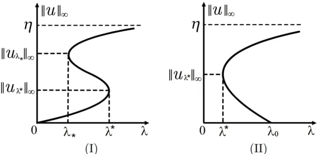
ExactlyS-shaped: We say that, on the (λ,kuk_∞)-plane, the bifurcation curve Sα is exactly S- shapedifSα isS-shaped and it hasexactly twoturning points; see Fig.1.1(I).

ReversedS-shaped: We say that, on the(λ,kuk_∞)-plane, the bifurcation curveS_αisreversed S- shapedifS_αhasat least twoturning points, say(λ^∗, ku_λ^∗k_∞)and(λ∗,ku_λ∗k_∞), satisfying λ∗ <λ^∗ andku_λ^∗k_∞ >ku_λ∗k_∞, and

(i) at(λ^∗,ku_λ^∗k_∞)the bifurcation curveSα turns to theleft, (ii) at(λ∗, kuλ∗k_∞)the bifurcation curveSα turns to theright,

(iii) S_α initially continues to theleftand eventually continues to theleft.

Exactly reversedS-shaped: We say that, on the (_λ,kuk_∞)-plane, the bifurcation curve S_α is exactly reversed S-shapedif Sα is reversedS-shaped and it has exactly twoturning points.

⊂-shaped: We say that, on the (λ,kuk_∞)-plane, the bifurcation curveSα is⊂-shapedif Sα has at least oneturning point, say(λ^∗,ku_λ^∗k_∞), satisfying

(i) at(λ^∗,ku_λ^∗k_∞)the bifurcation curveS_α turns to theright,

(ii) S_α initially continues to theleftand eventually continues to theright.

Exactly⊂_-shaped: We say that, on the (λ,kuk_∞)-plane, the bifurcation curve S_α is exactly

⊂-shapedifSα is⊂-shaped and it hasexactly oneturning point; see Fig.1.1(II).

Reversed⊂-shaped: We say that, on the(λ,kuk_∞)-plane, the bifurcation curveSαis⊂-shaped ifS_α hasat least oneturning point, say (λ^∗,ku_λ^∗k_∞), satisfying

(i) at(λ^∗,ku_λ^∗k_∞)the bifurcation curveS_α turns to theleft,

(ii) Sα initially continues to therightand eventually continues to theleft.

Exactly reversed⊂-shaped: We say that, on the(λ,kuk_∞)-plane, the bifurcation curve S_α is exactly reversed⊂-shapedifSα is reversed⊂-shaped and it hasexactly oneturning point.

In Section 2 below, we study the classification and evolution of bifurcation curves Sα of positive solutions for (1.1) with general nonlinearity f satisfying hypothesis (H). In addition, as applications, we study the classification and evolution of bifurcation curves S_α of positive solution for (1.1) with two particular nonlinearities

f(u) =exp u

1+εu

, ε>0 (1.6)

and

f(u) =u(1−_sinu) +u^p, p≥_{1 (1.7)}

Figure 1.1: (I) Exactly S-shaped bifurcation curve S_α with exactly two turn- ing points, which starts at (0, 0) and goes to infinity along the horizontal line kuk_∞ = η. (II) Exactly ⊂-shaped bifurcation curve Sα with exactly one turn- ing point, which starts at (λ₀, 0)and goes to infinity along the horizontal line kuk_∞ =η.

which satisfy hypothesis (H) withη=_∞.

Huang and Wang [6] studied the evolution and qualitative behaviors of bifurcation curves S¯ of positive solutions of one-dimensional perturbed Gelfand problem (1.2), (1.6).

Theorem 1.1 ([6, Theorem 2.1 and Fig. 1]). Consider (1.2), (1.6). Then there exists a positive

˜

ε≈0.2457such that, on the(λ,kuk_∞)-plane, such that the following assertions (i)–(iii) holds:

(i) For0<ε<ε, the bifurcation curve˜ S is exactly S-shaped.¯

(ii) Forε= ε, the bifurcation curve˜ S is strictly increasing and¯ (1.2),(1.6)has exactly one degenerate positive solution.

(iii) For ε > ε, the bifurcation curve˜ S is strictly increasing and all positive solutions of¯ (1.2), (1.6) are nondegenerate.

Wang [13] studied the evolution and qualitative behaviors of bifurcation curves ¯S of posi- tive solution of Dirichlet problem (1.2), (1.7).

Theorem 1.2([13, Theorem 2.1 and Figs. 1–2]). Consider(1.2),(1.7). Then, on the(_λ,kuk_∞)-plane, the bifurcation curveS satisfies the following assertions (i)–(iv).¯

(i) For p=1, the bifurcation curveS starts at¯ ^π₈², 0

and goes to infinity oscillationally along the vertical lineλ= ^π₈², and it has infinitely many turning points.

(ii) For1 < p < 2, the bifurcation curveS starts at¯ ^π₄², 0

and goes to infinity along the vertical lineλ=0, and it is reversed S-shaped.

(iii) For p = 2, the bifurcation curve S starts at¯ ^π₄², 0

and goes to infinity along the vertical line λ=0,and it is strictly decreasing.

(iv) For p > 2, the bifurcation curve S starts at¯ ^π₄², 0

and goes to infinity along the vertical line λ=0, and it is exactly reversed⊂-shaped.

The paper is organized as follows. Section2contains statements of main results. Section3 contains lemmas needed to prove the main results. Finally, Section 4 contains the proofs of the main results.

2 Main results

The main results in this paper are next Theorems 2.1–2.6 and 2.8. In Theorems 2.1 and 2.3 for (1.1), under (H) for nonlinearity f, for all α > 0, we present some basic properties of bifurcation curvesSα on the(λ,kuk_∞)-plane. In particular, in Theorem2.1(iii), we show that, on the(λ,kuk_∞)-plane,S_α moves to right strictly asαincreases andS_α tends to thekuk_∞-axis as αapproaches 0⁺ and tends to ¯Sas αapproaches infinity. In Theorem2.1(iv), we prove an interesting comparison result, cf. Remark 2.2 stated behind. In Theorems 2.4 and 2.5, under (H) and some suitable hypotheses on f, forα>0, we give a classification of bifurcation curves S_α on the (λ,kuk_∞)-plane. In Theorems 2.6 and2.8, as applications of Theorems2.1–2.5, we study the classification and evolution of bifurcation curves Sα for problem (1.2), (1.6) and problem (1.2), (1.7), respectively withαvarying from 0⁺to infinity.

We first define the numberλ^∗ =λ^∗(α)∈ 0,^π₄²

satisfying α=√

λ^∗tan√

λ^∗. (2.1)

Notice thatλ^∗ is a strictly increasing function ofα>_0.

Theorem 2.1. Consider (1.1) with fixed α > 0. Assume that f satisfies (H). Then the bifurcation curve S_αis a continuous curve on the(λ,kuk_∞)-plane. Moreover, on the(λ,kuk_∞)-plane, S_αsatisfies the following assertions (i)–(iv).

(i) If there exist s₀≥0and0< L₀ <_∞such that

ulim→0⁺

f(u) u^s0 = L₀,

then S_αstarts from infinity along the horizontal linekuk_∞ =0if s₀>1, from the point _2L^λ∗

0, 0 if s0=1, and from the origin(0, 0)if0≤s0 <1.

(ii) (a) Ifη=_∞and there exist s_∞ ≥0and0<L_∞ <_∞such that

ulim→_∞

f(u)

u^s∞ =L_∞, (2.2)

then S_α goes to infinity along the vertical lineλ=0if s_∞ >1, to infinity along the vertical line λ= _2L^λ∗

∞ if s_∞ =1, and to infinity asλ→_∞if0≤s_∞ <1.

(b) If0<η<_∞, f(η) =0and there exist s_η >0and L_η >0such that

ulim→η⁻

f(u)

(η−u)^sη = L_η,

then S_α goes to infinity along the horizontal linekuk_∞ = η if s_η ≥ 1, and ends at some point λ_η,η

withλ_η >₀if0< s_η <1.

(iii) For any two positive numbers α₁ < α₂, S_α2 lies strictly on the right hand side of S_α1 on the (λ,kuk_∞)-plane (So Sα₁∩Sα2 =∅). In addition,

(a) Asαapproaches0⁺, S_αtends to the positivekuk_∞-axis ifη=_∞and S_αtends to the segment (on the positivekuk_∞-axis) connecting the origin(0, 0)and the point(0,η)if0< η<_∞.

(b) Asαapproaches infinity, Sα tends toS.¯

(iv) (See Fig. 2.1.) Consider (1.1) with f = f₁ and f = f₂ both satisfying (H), and denote their bifurcation curves by S_α,1 and Sα,2respectively. If f2(u) ≥ f₁(u)for0 < u < η, then Sα,2 lies on the left hand side of (possibly coincides with) S_α,1 on the (λ,kuk_∞)-plane. In particular, if there exist two positive a<b<ηsuch that











f₂(u) = f₁(u) on

([0,a]∪[b,η] ifη<_∞, [0,a]∪[b,η) ifη=_∞, f₂(u)> f₁(u) on(a,b),

(2.3)

then, on the(_λ,kuk_∞)-plane, S_α,2coincide with S_α,1in the region

{(λ,kuk_∞):λ>₀and kuk_∞ ∈(0,a]∪[(α+₁)b,η)}

if(α+₁)b<ηand in the region

{(λ,kuk_∞):λ>0and kuk_∞ ∈(0,a]}

if (α+1)b ≥ η, and S_α,2 lies strictly on the left hand side of S_α,1 in the striped region {(λ,kuk_∞):λ>0and kuk_∞ ∈(a,b)}.

Figure 2.1: (I) Possible graphs of f₁ and f₂ satisfying f₁(u) = f₂(u) > 0 on [0,a]∪[b,∞)and f₂(u)> f₁(u)>0 on(a,b)with some positivea <b<η= _∞. (II) Possible corresponding bifurcation curves S_α,1 and Sα,2 on the (λ,kuk_∞)- plane.

Remark 2.2(Cf. Theorem2.1(iv) for Neumann–Robin problem (1.1)). Consider Dirichlet prob- lem (1.2) with f = f₁ and f = f₂ both satisfying (H) and (2.3), and denote their bifurcation

curves by ¯S₁and ¯S₂ respectively. Then it is well-known that, on the(λ,kuk_∞)-plane, ¯S₂ coin- cide with ¯S₁in the striped region{(λ,kuk_∞):λ>0 andkuk_∞ ∈(0,a]}and ¯S2 lies strictly on the left hand side of ¯S₁in the striped region{(λ,kuk_∞):λ>0 andkuk_∞ ∈(a,η)}.

Theorem 2.3. Consider(1.1). Assume that f satisfies (H). If f(u)−u f⁰(u) changes sign exactly k times in an interval(a,b)⊂(0,η)with some positive a< b≤η. Then there exist k positive numbers

(0<)α_k <· · · <α₂<α₁

such that, if0< α≤α_i for i∈ {1, 2, . . . ,k}, then the bifurcation curve Sαhas at least i turning points on the(λ,kuk_∞)-plane.

For the sake of convenience, we assume the following conditions.

(C1⁺) f(u)−u f⁰(u)≥ (6≡)0 on (0,β₁)with some β₁∈ (0,η). (C1⁻) f(u)−u f⁰(u)≤ (6≡)0 on (0,β₁)with some β₁∈ (0,η).

(C2⁺) If η = _∞, f(u)−u f⁰(u) ≥ (6≡) 0 on (β₂,η) with some β₂ ∈ (0,η). If η < _{∞, the} numbers_η defined in Theorem2.1(ii)(b) is equal to or larger than 1.

(C2⁻) Ifη=_∞, f(u)−u f⁰(u)≤(6≡)0 on (β₂,η)with some β₂ ∈(0,η). (D1) (See Fig.2.2(I).) There exist two positive p^∗ < _p <ηsuch that

f(u)−u f⁰(u)











>0, if 0<u< p^∗,

=0, ifu= p^∗ andu= p,

<0, if p^∗< u< p.

(D2) (See Fig.2.2(II).) There exist two positivep^∗ < p<ηsuch that

f(u)−u f⁰(u)











<0, if 0<u< p^∗,

=0, ifu= p^∗ andu= p,

>0, if p^∗< u< p.

Theorem 2.4. Consider(1.1). Assume that f satisfies (H). Then, on the(_λ,kuk_∞)-plane, the bifurca- tion curve Sα satisfies the following assertions (i)–(iv).

(i) If f(u)−u f⁰(u)>0(resp. f(u)−u f⁰(u)<0) almost everywhere for u>0, then S_αis strictly increasing (resp. strictly decreasing) for allα>0.

(ii) If f(u)satisfies (C1⁺), (C2⁺) and (D1) (resp. (C1⁻), (C2⁻) and (D2)) with positive p^∗ < p<η andRp

0 s[f(s)−s f⁰(s)]ds <0 (resp. Rp

0 s[f(s)−s f⁰(s)]ds > 0). Then Sα is S-shaped (resp.

reversed S-shaped) for allα>0.

(iii) (See Fig. 2.3.) If f(u) satisfies (C1⁺), (C2⁺) and (D1) (resp. (C1⁻), (C2⁻) and (D2)) with positive p^∗ < p< ηand the following conditions (3a)–(3b) hold.

(3a) The bifurcation curveS of¯ (1.2)is S-shaped (resp. reversed S-shaped),

Figure 2.2: (I) Graph of 2F(u)−u f(u)satisfying condition (D1). (II) Graph of 2F(u)−u f(u)satisfying condition (D2).

(3b) p^∗ <ku_λ1k_∞ < p<ku_λ2k_∞where λ₁,ku_λ1k_∞and λ₂,ku_λ2k_∞are turning points of S such that¯ S turns to the left (resp. to the right) at¯ λ₁,ku_λ1k_∞andS turns to the right¯ (resp. to the left) at λ2,ku_λ2k_∞.

Then S_α is S-shaped (resp. reversed S-shaped) for all α > 0. Furthermore, there exist two points λ₃,ku_λ3k_∞ and λ₄,ku_λ4k_∞ on Sα such that ku_λ3k_∞ ≤ ku_λ1k_∞ < p ≤ ku_λ4k_∞ and the portion of S_α connecting λ₃,ku_λ3k_∞and λ₄,ku_λ4k_∞ is monotone decreasing (resp.

monotone increasing), where λ₃,ku_λ3k_∞is a turning point to the left (resp. to the right) of S_α and λ₄,ku_λ4k_∞is a turning point to the right (resp. to the left) of Sα.

(iv) If f(u)satisfies (C1⁻) and (C2⁺) (resp. (C1⁺) and (C2⁻)), then Sα is ⊂-shaped (resp. reversed

⊂-shaped) for allα>0.

Theorem 2.5. Consider(1.1). Assume that f satisfies (H). Then, on the(λ,kuk_∞)-plane, the bifurca- tion curve Sα satisfies the following assertions (i)–(iii).

(i) If f(u) satisfies (C1⁺) and (C2⁺) and f(p˜)−p f˜ ⁰(p˜) < 0 with some p˜ ∈ (0,η), then S_α is S-shaped forα>0small enough.

(ii) If f(u) satisfies (C1⁻) and (C2⁻) and f(p˜)−p f˜ ⁰(p˜) > 0 with some p˜ ∈ (0,η), then Sα is reversed S-shaped forα>0small enough.

(iii) Assume that f(u) satisfies (C1⁺) (resp. (C1⁻)) with some β₁ ∈ (0,η), the bifurcation curve S of¯ (1.2) is strictly increasing (resp. strictly decreasing) on the (λ,kuk_∞)-plane, and (1.2) has no degenerate solution. Then, on the(_λ,kuk_∞)-plane, for everyρ₀ ∈ (β₁,η), there exists α^∗ =α^∗(ρ₀)>0such that, forα≥ α^∗,Sαis strictly increasing (resp. strictly decreasing) in the striped region{(λ,kuk_∞):λ>0and kuk_∞ ∈(0,ρ₀]}. In addition, assume that there exists a constantρ¯₀ ∈(β₁,η)such that

0<θ(u)<θ(ρ¯₀)<θ(u¯₁)<θ(u¯₂) for0< u<ρ¯₀ <u¯₁ <u¯₂ <_{η, (2.4)}

Figure 2.3: Illustration of S-shaped bifurcation curves S_α and ¯S in Theorem 2.4(iii).

(resp.

0>θ(u)>θ(ρ¯₀)>θ(u¯₁)>θ(u¯₂) for0< u<ρ¯₀ <u¯₁ <u¯₂ <η), (2.5) where θ(x) ≡ 2Rx

0 f(s)ds−x f(x). Then, for α ≥ α^∗, S_α is strictly increasing (resp. strictly decreasing) on the(λ,kuk_∞)-plane.

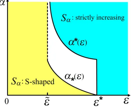
Theorem 2.6(See Fig.2.4.). Consider(1.1),(1.6). Suppose that ε∗ ≡ ¹

4.25 (≈0.235)<ε˜<ε^∗ ≡ ¹

4 =0.25,

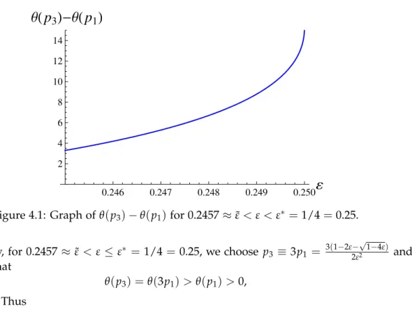
where the number ε˜ ≈ 0.2457 exists in Theorem 1.1. Then, on the (λ,kuk_∞)-plane, the bifurcation curve S_α satisfies the following assertions (i)–(iii).

(i) For0< ε<ε, S˜ α is S-shaped for allα>0.

(ii) (a) Forε˜ ≤ε<ε^∗, S_α is S-shaped for0<α≤α∗(ε)≡ ^p_p²

1 −₁where p₁= ¹−2ε−√

1−4ε

2ε² < p₂= ¹−2ε+√ 1−4ε

2ε² ,

are two positive zeros of quadratic polynomialε²u²+ (2ε−1)u+1.The termα∗(ε) = ^p_p²

1 −1=

2√ 1−4ε 1−2ε−√

1−4ε is a strictly decreasing function ofε ∈(ε,˜ ε^∗)and satisfies lim

ε→(ε˜)⁺

α∗(ε)≈1.690 and lim

ε→(ε^∗)⁻

α∗(ε) =0. (2.6)

(b) Forε˜<ε<ε^∗, Sα is strictly increasing forα≥α^∗(ε)with someα^∗(ε)>0.

(iii) For ε≥ε^∗, S_α is strictly increasing for allα>0.

Figure 2.4: Classification of bifurcation curvesSα on the first quadrant of(ε,α)- plane for Theorem2.6.

Conjecture 2.7. We conjecture that, in Theorem2.6(ii) for(1.1),(1.6), when ε= ε˜≈ 0.2457, on the (λ,kuk_∞)-plane, the bifurcation curve S_α is S-shaped forallα>0.Further investigation is needed.

Theorem 2.8(Cf. Theorem1.2for (1.2), (1.7)). Consider(1.1),(1.7). Then, on the(λ,kuk_∞)-plane, the bifurcation curves S_α satisfies the following assertions (i)–(iv).

(i) For p=1, Sα has infinitely many turning points for allα>0.

(ii) For1< p<2, for any positive integer k, there exist k positive numbers (0<)α_k <· · ·< α₂<α₁

such that Sα has at least i turning points for0<α≤α_ifor i ∈ {1, 2, . . . ,k}. (iii) For p=2, S_α is strictly decreasing for allα>0.

(iv) For p>2, Sα is⊂-shaped for allα>0.

Remark 2.9. For 1.9 ≤ p ≤ 2, numerical simulations show that the bifurcation curve ¯S for Dirichlet problem (1.2), (1.7) is strictly decreasing on the (λ,kuk_∞)-plane, cf. [13, Fig. 2].

However, by Theorem2.8 (ii), on the(λ,kuk_∞)-plane, the bifurcation curveS_αfor Neumann–

Robin problem (1.1), (1.7) can have arbitrarily many turning points as desired for α > 0 small enough.

3 Lemmas

To prove our main results for one-dimensional Neumann–Robin problem (1.1), we develop some new time-map techniques which time-map technique was used in Anuradha, Maya,

and Shivaji [4]. We first define the following functions F(u) =

Z _u

0 f(s)ds, G(m,ρ) =

Z _ρ

m α

ds

pF(ρ)−F(s)^{, H}(m,ρ) = _q ^m F(ρ)−F(^m

α)

, (3.1)

where ρ ≡ u(0) = kuk_∞ > 0 and m ≡ −u⁰(1) = αu(1) ∈ (0,αu(0)) = (0,αρ), see [4, pp.

95–97]. We have the following properties for functionsGandH in the next lemma.

Lemma 3.1([4, Section 2 and Theorem 2.1]). Consider(1.1). Assume that f satisfies (H). Then the following assertions (i)–(iii) hold.

(i) For fixedρ>0, G(m,ρ)is a strictly decreasing function of m on(0,αρ). Furthermore

mlim→0⁺G(m,ρ) =

Z _ρ

0

ds

pF(ρ)−F(s) >0 and lim

m→(αρ)⁻

G(m,ρ) =0.

(ii) For fixedρ>0, H(m,ρ)is a strictly increasing function of m on(0,αρ). Furthermore

mlim→0⁺H(m,ρ) =0 and lim

m→(αρ)⁻

H(m,ρ) =_∞.

(iii) For anyρ>0, there exits a unique m =mρ =mα,ρ∈ (0,αρ)such that G(mρ,ρ) = H(mρ,ρ). (Later, for simplicity, we usually write m_ρinstead of m_α,ρ unless necessary.)

By Lemma 3.1(iii), we see that, ifu(0) = kuk_∞ = ρ > 0, then (1.1) has a unique positive solution u. Since u⁰(₁) +αu(₁) = 0, we have that u⁰(₁) = −m_ρ < _{0 and} u(₁) = ^mρ

α > _{0; see} [4, p. 96]. Furthermore, we define thetime-map functionfor one-dimensional Neumann–Robin problem (1.1)

T(ρ) =

Z _ρ

mρ α

ds

pF(ρ)−F(s) = _q ^mρ F(ρ)−F(^mρ

α )

. (3.2)

Then by [4, Theorem 2.1],

T(ρ) = q

2λ(ρ), (3.3)

and hence by (1.4), we have the bifurcation curve of positive solutions for (1.1) Sα =

1

2[T(ρ)]²,ρ

:ρ∈(0,η)

. (3.4)

We also define thetime-map functionfor one-dimensional Dirichlet problem (1.2) T¯(ρ) =

Z _ρ

0

ds

pF(ρ)−F(s)^{, (3.5)}

and we have similar results that

T¯(ρ) = q

2λ(ρ)

and by (1.5) the bifurcation curve of positive solutions for (1.2) S¯ =

1

2[T^¯(ρ)]²,ρ

:ρ∈ (0,η)

; (3.6)

see e.g. [6, Eq. (11)].

Lemma 3.2. Consider(1.1). Fixρ (= u(0))> 0and consider ^m_α^ρ (= u(1))as a function ofα > 0.

Then the following assertions (i)–(iii) hold.

(i) ^m_α^ρ is strictly decreasing on(0,∞), lim_α→0^{+ m}_α^ρ = ρ,andlim_α→_∞ ^m_α^ρ =0.

(ii) For eachα>₀andρ∈(_0,η)_, ρ

α+1 < ^mρ

α < ρ (that is, u(0)

α+1 <u(1)< u(0)). (3.7) (iii) For s₀≥0defined in Theorem2.1(i) and s_∞ ≥0defined in Theorem2.1(ii) (a) withη=_∞,

lim

ρ→0⁺

mρ

αρ <1 (3.8)

and

lim

ρ→_∞

m_ρ

αρ <1. (3.9)

Proof. (I)First, we rewrite functions HandGin (3.1) as functions ofα, ^m_α = ^mρ

α = ^mα,ρ

α

=k andρ, and we obtain that

G=G(α,k,ρ)≡

Z _ρ

k

ds pF(ρ)−F(s)^, H =H(_α,k,ρ)≡ _q ^m

F(ρ)−F(^m

α)

= _p ^k

F(ρ)−F(k)×_α.

We see that, for fixedk, G(α,k,ρ)is constant in α, butH(α,k,ρ)is linear inα. Ifα=α₀, we let k₀≡ ^mα0,ρ

α0 and

G(α₀,k₀,ρ) =

Z _ρ

k₀

ds

pF(ρ)−F(s) = H(α₀,k₀,ρ) = _p ^k0

F(ρ)−F(k₀)×α₀. Takingα> α₀, we have that

G(α,k₀,ρ) =

Z _ρ

k0

ds

pF(ρ)−F(s) = G(α₀,k₀,ρ)< H(α,k₀,ρ) = _p ^k0

F(ρ)−F(k₀)×α.

Then by Lemma3.1(i)–(ii), for α> α₀, we obtain that ^m_α^α,ρ = k_ρ <k₀ = ^mα0,ρ

α0 . So ^m_α^ρ is strictly decreasing on(0,∞).

Secondly, given anyε>0, we have that G(α,ρ−ε,ρ) =

Z _ρ

ρ−ε

ds

pF(ρ)−F(s) >0 and H(α,ρ−ε,ρ) = ^ρ−ε

pF(ρ)−F(ρ−ε)×α>0.

For

0< α<δ ≡ Rρ

ρ−ε

√ ds

F(ρ)−F(s) ρ−ε

√

F(ρ)−F(ρ−ε)

, we have that

H(α,ρ−ε,ρ) = ^ρ−ε

pF(ρ)−F(ρ−ε)×α<

Z _ρ

ρ−ε

ds

pF(ρ)−F(s) =G(α,ρ−ε,ρ).

By Lemma 3.1(i)–(ii), for 0 < α < δ, we see that ρ−ε < ^mρ

α = k < ρ, which proves that lim_α→0⁺

mρ

α =ρ. Similarly, we can prove that limα→_∞ ^m_α^ρ =0. The proof of part (i) is complete.

(II)By Lemma3.1(iii), we have that(0<) ^mρ

α <ρ, which also follows from (1.3). Thus we are left to prove that _α+^ρ₁ < ^mρ

α . By (3.2), we have that m_ρ=

Z _ρ

mρ α

q

F(ρ)−F(^m_α^ρ) pF(ρ)−F(s) ^ds>

Z _ρ

mρ α

ds=ρ− ^mρ α , which is equivalent to _α+^ρ₁ < ^m_α^ρ. So part (ii) holds.

(III)The proof of part (iii) is easy but tedious and hence we put it in AppendixA.

The proof of Lemma3.2is complete.

Lemma 3.3. Consider(1.1)and assume that f satisfies (H). Then, for fixedα>0, mρis a C³function forρ>0and

m⁰_ρ ≡ ^∂

∂ρm_ρ=

2^m_αρ^ρ +P D(^mρ

α ) +m_ρf(ρ) 2 ¹_α +1

D(^mρ

α ) +^mρ

α f(^mρ

α )^{, (3.10)}

where

θ(x)≡2F(x)−x f(x), D(x)≡ F(ρ)−F(x), P≡ ¹ ρ

Z _ρ

mρ α

q D(^mρ

α )

D³²(s) [θ(ρ)−θ(s)]ds. (3.11) In addition,

T⁰(ρ)≡ ^∂

∂ρT(ρ) = ^∆(ρ)

Φ(ρ)^{, (3.12)}

where

∆(ρ) =Ph Dm_ρ

α

+^mρ 2αfm_ρ

α i

+^mρ αρ

h

θ(ρ)−θ m_ρ

α i

, (3.13)

Φ(ρ) = r

Dm_ρ α

2

1 α

+₁

Dm_ρ α

+^mρ α fm_ρ

α

>_{0. (3.14)} The proof of Lemma3.3is easy but tedious and hence we put it in AppendixB.

By (3.12)–(3.14) and (3.2), we see that, if θ(ρ)−θ(s)does not change sign fors ∈ ^m_α^ρ,ρ , then we can determine the sign ofT⁰(ρ). Furthermore, by Lemma3.2(ii), it suffices to consider the interval _α+^ρ₁,ρ

since _α+^ρ₁ < ^mρ

α . We state this result in the following lemma.

Lemma 3.4. Consider(1.1)and assume that f satisfies (H). Then, for fixedα>0and for u∈ ^ρ

α+1,ρ andρ∈(0,η),

T⁰(ρ)

(>0, ifθ(ρ)−θ(u)≥(6≡)0,

<0, ifθ(ρ)−θ(u)≤(6≡)0.

Remark 3.5. Lettingα→_∞in (3.12), by Lemma3.2(i), the time-map ¯T(ρ)for (1.2) satisfies T¯⁰(ρ)≡ ^∂

∂ρ

T¯(ρ) = ¹ 2ρ

Z _ρ

0

θ(ρ)−θ(s) [D(s)]^{3/2 ds.}

And similarly, foru∈ (0,ρ),

T¯⁰(ρ)

(>_{0, if}θ(ρ)−θ(u)>_0,

<0, ifθ(ρ)−θ(u)<0.

Lemma 3.6. Consider(1.1)with fixedα>0.For f(u) = u^bwith b ≥0, T(ρ)satisfies the following assertions (i)–(iii).

(i) If b>1, thenlim_ρ→0⁺T(ρ) =_∞,limρ→_∞T(ρ) =0,and T⁰(ρ)<0forρ∈ (0,∞). (ii) If b =1, then T(ρ)≡√

λ^∗on (0,∞), whereλ^∗ ∈(0,^π₄²)is defined in(2.1).

(iii) If0≤b<1, thenlim_ρ→0⁺T(ρ) =0,limρ→_∞T(ρ) =_∞,and T⁰(ρ)>₀forρ∈ (0,∞). Proof. (I)First, for f(u) =u^b withb≥0, we calculate that

F(u) = ¹ b+₁^u

b+1,

D(u) =F(ρ)−F(u) = ¹

b+1ρ^b+1− ¹

b+1u^b+1, θ(u) =2F(u)−u f(u) = ¹−b

b+1u^b+1, θ(ρ)−θ(u) = ¹−b

b+1ρ^b+1−¹−b

b+1u^b+1= (1−b)D(u). We observe that

D(u) = ¹

b+₁(ρ^b+1−u^b+1)∈ u^b

b+₁(ρ−u), ρ^b+1 b+₁

forρ >u, (3.15)

P= ¹ ρ

Z _ρ

mρ α

q D(^mρ

α )

D³²(s) [θ(ρ)−θ(s)]ds

= ¹ ρ

Z _ρ

mρ α

q D(^mρ

α )

D³²(s) (1−b)D(s)ds= ¹

ρ(1−b) r

D(^mρ α )T(ρ). Forb≥0, by (3.15), we have that

T(ρ) =

Z _ρ

mρ α

ds pD(s) ≥

√b+1 ρ^b

+1 2

ρ

1− ^mρ αρ

=

√b+1 ρ

b−1 2

1− ^mρ

αρ

. (3.16)

On the other hand, by (3.15), we have that T(ρ) =

Z _ρ

mρ α

ds pD(s) ≤

√b+1 _m

ρ

α

^b₂ Z _ρ

mρ α

√ds ρ−s

≤ ²

√b+1 _m

ρ

α

^b₂ r

ρ−^mρ α ≤2√

b+1(α+1)^b2 v u u t

1− ^mρ

αρ

ρ^b−1 . (3.17)

Then, since b>1 and by Lemma3.2(iii), we have that lim_ρ→0⁺T(ρ) = _∞and lim_ρ→_∞T(ρ) = 0. In addition, by (3.12)–(3.14), the numerator ofT⁰(ρ)is

∆(ρ) = ¹ 2

hm_ρ α fm_ρ

α

+2Dm_ρ α

i

P+ ^mρ αρ

h

θ(ρ)−θ m_ρ

α i

= ¹ 2

m_ρ α

b+1

+2Dm_ρ α

1−b

ρ r

Dm_ρ α

T(ρ) + ^mρ

αρ (1−b)Dm_ρ α

= (₁−b) ( 1

2ρ m_ρ

α b+1

+_2D^mρ α

r D

m_ρ α

T(ρ) + ^mρ αρD

m_ρ α

)

(3.18)

<0

since b>1. ThusT⁰(ρ)<0 forρ∈ (0,∞). So part (i) holds.

(II)We prove part (ii). For f(u) =u, we computeT(ρ)in (3.2) and we have that T(ρ) =

Z _ρ

mρ α

ds q1

2ρ²− ¹₂s²

= _r ^mρ

1

2ρ²− ¹₂^mρ

α

2. (3.19)

So we obtain that

arccos mρ

αρ

=

mρ

αρ

r

1−^mρ

αρ

2 ×α, (3.20)

which holds for every ρ > 0, with positive αfixed. Thus ^m_αρ^ρ is constant in ρ. By (3.3), if we consider√

λ∈ (0,^π₂)as an angle of a triangle and ^m_αρ^ρ as its cosine value in the triangle, then

tan

√ λ=

r

1−^mρ

αρ

2 mρ

αρ

and√

λtan√

λ=αby (3.19)–(3.20). SoT(ρ)≡√

λ^∗, whereλ^∗ ∈(0,^π₄²)is defined in (2.1). So part (ii) holds.

(III)Part (iii) for f(u) =u^bwith 0≤b<1 follows easily by applying (3.16)–(3.18).

The proof of Lemma3.6is complete.

Lemma 3.7. Consider(1.1)with s₀, s_∞, L₀, and L_∞defined in Theorem2.1(i)–(ii). Then the following assertions (i) and (ii) hold:

(i) There exists a function R0(ρ)such that T(ρ) =

Z _ρ

mρ α

[1+R0(ρ)]ds q L0

s0+1ρ^s0+1− _s^L0

0+1s^s0+1 ,

wherelim_ρ→0⁺R₀(ρ) =0.

(ii) There exists a function R_∞(ρ)such that T(ρ) =

Z _ρ

mρ α

[1+R_∞(ρ)]ds q L_∞

s_∞+1ρ^s∞+1− _s^L∞

∞+1s^s∞+1 ,

wherelimρ→_∞R_∞(ρ) =0.

Proof. We simply prove part (ii). The proof of part (i) is similar. We compute that T(ρ) =

Z _ρ

mρ α

ds pF(ρ)−F(s)

=ρ Z ₁

mρ αρ

L_∞ s_∞+₁

h

ρ^s∞+1−(ρs)^s∞+1i+

Z _ρ

ρs f(u)−L_∞u^s∞du −1/2

ds

=ρ Z ₁

mρ αρ

L_∞ s_∞+₁

h

ρ^s∞+1−(ρs)^s∞+1i

−1/2"

1−

p1+φ(ρ,s)−1 p1+φ(ρ,s)

# ds, where

φ(ρ,s) = Rρ

ρsf(u)−L_∞u^s∞du

L∞

s_∞+1[ρ^s∞+1−(ρs)^s∞+1]^. Sinces≥ ^mρ

αρ > ¹

α+1, we have that 0≤ |φ(ρ,s)|=

Rρ

ρs f(u)−L_∞u^s∞du

L_∞

s_∞+1[ρ^s∞+1−(ρs)^s∞+1]

≤

Rρ ρsu^s∞du

L_∞

s_∞+1[ρ^s∞+1−(ρs)^s∞+1]_t∈(^sup_α+^ρ1,ρ)

f(t) t^s∞ −L_∞

= ¹

L_∞ sup

t∈(_α+^ρ1,ρ)

f(u) t^s∞ −L_∞

.

We see thatφ(ρ,s)approaches zero asρ→∞, uniformly ins. So R_∞(ρ)≡ −

p1+φ(ρ,s)−1

p1+φ(ρ,s) →0 asρ→_∞, and hence part (ii) holds.

The proof of Lemma3.7is complete.

Lemma 3.8. Consider(1.1) with s₀, s_∞, L₀, and L_∞ defined in Theorem2.1(i)–(ii) andλ^∗ defined in (2.1). Then

lim

ρ→0⁺T(ρ) =











∞, if s₀>1, q

λ^∗

L0, if s₀=1, 0, if0≤s₀<1,

(3.21)

lim

ρ→_∞T(ρ) =











0, if s_∞>1, q

λ^∗

L_∞, if s_∞=1,

∞, if0≤s_∞<_1.

(3.22)

Proof. If s₀ ≥ 0 and s₀ 6= 1, Eq. (3.21) follows by Lemmas 3.6 and3.7. If s₀ = 1, we rewrite (1.1) as

−u⁰⁰(x) =λf(u(x)) = [L₀λ]

f(u(x)) L0

=λ^˜ f˜(u(x))_, with ˜λ ≡ L₀λ and ˜f(u) ≡ ^f_L^(u)

0 . Then lim_u→0⁺ f˜(u)

u = _limu→0+ f(u)

uL0 = 1, and we can apply Lemmas3.6and3.7to get lim_ρ→0⁺T(ρ) =^qλ_L^∗

0. The proof of Eq. (3.21) is complete. Eq. (3.22) can be proved similarly. We omit it here.

The proof of Lemma3.8is complete.