The paper has appeared in Journal of Chemometrics wileyonlinelibrary.com/journal/cem

(1)

The paper has appeared in Journal of Chemometrics wileyonlinelibrary.com/journal/cem

How to cite this article: Héberger K, Kollár‐Hunek K. Comparison of validation variants by sum of ranking differences and ANOVA. Journal of Chemometrics. 2019;e3104.

https://doi.org/10.1002/cem.3104

Comparison of validation variants by sum of ranking differences and ANOVA

Károly Héberger¹ and Klára Kollár-Hunek²

1 Plasma Chemistry Research Group, Research Centre for Natural Sciences, Hungarian Academy of Sciences, H-1117 Budapest, Magyar tudósok krt. 2, Hungary;

2 Department of Inorganic and Analytical Chemistry, Budapest University of Technology and Economics, H-1111 Budapest, Szt. Gellért tér 4, Hungary

* To whom correspondence should be addressed:

Károly Héberger,

Research Centre for Natural Sciences, Hungarian Academy of Sciences H-1117 Budapest XI., Magyar tudósok krt. 2

H-1519 Budapest, P. O. Box. 286, Hungary Phone: +36 1 382 65 09

Email: heberger.karoly@ttk.mta.hu

(2)

-2- Abstract

The old debate is revived: definite differences can be observed in suggestions of estimation for prediction performances of models, and for validation variants according to the various scientific disciplines. However, the best and/or recommended practice for the same data set cannot be dependent on the field of usage. Fortunately, there is a method comparison algorithm, which can rank and group the validation variants; its combination with variance analysis will reveal whether the differences are significant or merely the play of random errors. Therefore, three case studies have been selected carefully to reveal similarities and differences in validation variants. The case studies illustrate the different significance of these variants well. In special circumstances any of the influential factors for validation variants can exert significant influence on evaluation by sums of (absolute) ranking differences (SRDs): stratified (contiguous block) or repeated Monte Carlo resampling, and how many times the data set is split (5-7-10). The optimal validation variant should be determined individually again and again. A random resampling with sevenfold cross- validations seems to be a good compromise to diminish the bias and variance alike. If the data structure is unknown, a randomization of rows is suggested before SRD analysis. On the other hand, the differences in classifiers, validation schemes, and models proved to be always significant and even subtle differences can be detected reliably using SRD&ANOVA.

Keywords: Model validation, cross-validation; resampling, method comparison, ranking

(3)

-3- 1. INTRODUCTION

In recent years several variants of model validation have been introduced and their predictive performance is investigated:

i) Randomization test, also called permutation test i.e. shuffling of Y values.¹

ii) Split of the data into three parts: training, (learning) set or analysis sample, monitoring (calibration) set, prediction (test) set.² An external test set guarantees larger generalizability even if, it cannot select the “best” possible model(s).^3,4

iii) Cross-validation (CV): leave-one-out, leave-n-out, double CV, etc.^5-7

Herewith we cannot recapitulate the whole discussion, but some key points are referred below:

“If possible, an independent sample should be obtained to test the adequacy of the prediction equation. Alternatively, the data set may be divided into three parts; one part to be used for model selection [model building or variable selection], the second part for the calibration of parameters in the chosen model and the last part for testing the adequacy of predictions”.²

Cross-validation is perhaps the most widely used method for estimating prediction error;

however, it is debatable how well cross-validation can reveal the prediction performance. Various implementations of cross-validation inherently call for a compromise in terms of the bias-variance trade-off. As Hastie, Tibshirani and Friedman point out, “[…] five- or ten-fold cross-validation will overestimate the prediction error. Whether this bias is a drawback in practice depends on the objective. On the other hand, leave-one-out cross-validation has low bias, but can have high variance. Overall, five- or tenfold cross-validation are recommended as a good compromise”.⁵

Recently more and more evidences suggest that 10-fold cross-validation is a viable option, Gütlein et al. maintain that “contrary to current conception in the community, cross-validation may play a significant role in evaluating the predictivity of (Q)SAR models”.⁶

Kohavi in his highly cited paper has compared two classifiers on real world examples. The number of folds has been varied in k-fold cross-validation and also whether the CV was stratified or not. The number of bootstrap samples was also varied, and established that a ten-fold stratified cross-validation is the best method and maybe better than the more calculation-demanding leave- one-out cross-validation.⁷

Unfortunately, the same techniques are often called differently in different disciplines and many validation techniques can be realized in different ways. The word “resampling” is misleading in chemistry as no new samples are measured, but a distribution is rendered to statistical parameters

(4)

-4-

by using the original data with re-sampling them in the statistical sense. Additionally, it can be completed with or without repetitions, and is called Monte Carlo resampling or k-fold cross- validation, respectively. Even the latter one can be carried out differently: Venetian blinds (123,123,123, etc.), contiguous blocks (111,222,333, etc.), random selection (e.g. 1132213332, etc.), where 1, 2, and 3 denotes the training, the validation, and the test sets.⁸

The large number of validation variants can be ranked and grouped, and used for establishing the predictivity of models, still some questions arise immediately, which ones are the best, and which ones should be avoided? Which ones are equivalent or significantly different and at which circumstances? Therefore, we carried out a large-scale comparison of validation variants using three emblematic data sets with known, but deviating properties. Fortunately, the procedure based on sum of (absolute) ranking differences (SRDs) is suitable for a detailed method comparison.

Analysis of variance (ANOVA) is able to decompose the effects of different factors (see later).

One of the unknown reviewers pointed out that cross-validation (CV) might be carried out with different aims: “i) to compare models for hyperparameter tuning or ii) to estimate unbiasedly the prediction error.” Accordingly, different algorithms and behavior are expected, though most sources do not mention, which variants are considered for model building or for estimation of the prediction error (also called generalizability); eventually both. To avoid any confusion, we state that our examinations are sheer comparisons of validation variants from the point of view of the prediction error. Case study No 2. applies cross-validation (and single split) resampling methods for model building (but claim generalizability) and we compared them concerning predictivity.

2. MATERIALS AND METHODS 2.1 Description of SRD procedure

Sum of ranking differences (SRD) is a relatively new and rapidly expanding technique for method comparison.^9,10 The SRD algorithm is entirely general and allows ranking, grouping variables and automatic selection of a set of variables. Y.-Z. Liang et al. find SRD as “a simple objective procedure”.¹¹ The background philosophy is indeed quite simple and similar to that for round-robin tests (proficiency testing): The systematic errors (biases) of different laboratories and/or different measurement techniques follow normal distribution. Naturally, there is no theoretical proof for that, but it is a well-substantiated empirical finding in analytical chemistry.

(5)

-5-

At least the laboratories and techniques are compared using Z-scores with the assumption of normality.¹²

The items (i.e. variables) to be compared should be arranged in the columns and the objects (data sets, error rates, compounds etc., i.e. samples,) are arranged in the rows of the input matrix.

The SRD technique is supervised in the sense that it requires some gold standard (benchmark or a reference) for ranking. The reference is used for data fusion as summarized by Willett¹³ and should be selected according to the nature of the data. Perhaps the most frequently applied data fusion possibility is the usage of average. The arithmetic mean ensures that the random errors cancel each other out. The maximum likelihood principle justifies the usage of the most probable value instead of any individual one. It is also called consensus approach (modeling).¹⁴ Other data fusion options also exist, for example row minimum for error rates, residuals, misclassification rates, etc. row maximum is a suitable gold standard for the best classification rates, explained variance and so on.

Row maxima and minima are valid in the case of properties that are maximized or minimized under optimal conditions.

1) STEP 1 is a data fusion act: definition of a gold standard (benchmark) depending on the features of the data set; it can be the average: (arithmetic mean), or median (for asymmetric distributions, in the presence of outliers), minimum, maximum, a known standard, etc. The input data table for case study No 1 encloses misclassification rates, i.e. the natural selection of the reference is the row minimum. It is equivalent to the selection of the hypothetical best possible classifier, which produces the smallest misclassification rates for each data sets. Similarly, minimum was selected for standard deviations, biases and mean squared error for case study No 2. Average of modeled and experimental retention indices was applied as reference for case study No. 3.

2) STEP 2 is column by column the evaluation of index vectors, the calculation of (absolute) differences between standard and individual vector coordinates and adding the differences for each object (samples, row designee) together. These values are called as SRD values and rank the individual variables (column designee). The smaller the SRD the closer the variable is to the benchmark, i.e. the better. The mutual proximity of SRD values indicates the specific grouping of variables. Because the coordinates of the columns cannot always be strictly monotonously ordered, the way of determining the index vectors' coordinates is known as ranking with ties. The

(6)

-6-

normalized SRD values (scaled between 0 and 100) are then plotted, together with the distribution of SRD values for randomized rank numbers. The details are given in our earlier work.¹⁵

3) STEP 3 involves two validation steps: permutation test (denoted by CRNN = comparison of ranks with random numbers) and cross-validation. (The latter is the collective name of several similar techniques, see later.) For convenience SRD values are normalized between 0 and 100 to obtain comparability between various data sets. A detailed description of the SRD technique can be found in our earlier work¹⁶ along with a summarizing animation of the process as an additional file 3 in ref.¹⁶ SRD is developed as an MS Excel macro, and is available for download at:

http://aki.ttk.mta.hu/srd

Recent sources^17,18 clearly show that the SRD is not simply a distance metric, but a composite procedure including data fusion and validation steps, as well. Moreover, SRD realizes a multicrieria (multiobjective) optimization, as it ranks and detects the possible groupings of similar solutions of the Pareto front that match the decision maker’s preferences. This way the SRD technique provides a smaller set of optimal solutions.¹⁹

2.2 SRD value as measure for bias

The SRD values can be considered as a bias measure: its definition is:^9,10,15 𝐵𝑖𝑎𝑠 = ∑|𝑟_𝑖 − 𝑞_𝑖|

𝑛

𝑖=1

(1) where 𝑟_𝑖= rank number of object i for the actual cross-validation method

𝑞_𝑖= rank number object i for the benchmark reference (average).

2.3 Variance measures for SRD values

As it was outlined in the introduction the variance measure may depend on the way of (cross-) validation (from here on, validation variants). The term “cross-validation” is not quite proper here as no prediction (test) set exists and used for checking. In all SRD analysis k-fold cross-validation (k=5, 7 and 10) was realized in a stratified manner (contiguous blocks, case A) and in a Monte Carlo way (leave-many-out repeated resampling, case B). Respectively, roughly 1/5^th, 1/7^th, and 1/10^th of the rows were left out and the SRD procedure was repeated on the remaining 4/5^th, 6/7^th and 9/10^th part of the input matrix. Then, this ranking was repeated as many times as it is determined by dP=nR\rPd and by nR\dP, where nR is the number of rows in the input matrix, rPd

(7)

-7-

is the rate of parts to delete (5, 7 or 10), i.e., dP is the number of rows to delete (see the manual in the supplementary information 1). Such a way uncertainties (variances) were assigned to each SRD attribute. These variances overestimate the true prediction error in case of k-fold cross-validation (conservative estimation). Our earlier program¹⁵ was completed with the above validation options.

The user manual can be found in the supplementary material 1.

2.4 ANOVA

Analysis of variance (ANOVA) was used for the comparison of above validation variants using the SRD values. This method is based on the pairwise comparison of the average values of the different groups of samples. The following factors were defined: F1 - way of cross-validation, two levels: contiguous and resampling; F2 - number of folds, three levels: 5-, 7- and 10-fold and F3–

methods to be compared, classifiers (case study 1, 13 levels); resampling methods (case study 2, seven levels); models predicting retention indices (case study 3, 25 levels) The different factors were compared separately. STATISTICA 13 (Dell Inc., Tulsa, OK, USA) was used for the analysis.

2.5 Data sets

Three different data sets with various idiosyncrasies were carefully selected for the comparison and for studying the bias and variance trade off.

2.5.1 Case study number 1. Comparison of classifiers

Cannings & Samworth recently introduced a new technique called “Random-projection ensemble classifier”²⁰ (RPEC). The authors introduced a general framework for high dimensional classification on carefully selected low dimensional random projections. Each random projection can be considered as a perturbation of the original data and it is thought that the ‘stable’ effects that are sought by statisticians are found. They focused their research on the classification performance of RPEC and misclassification rates were selected for comparison of the following classifiers: Base ones: linear discriminant analysis (LDA), quadratic discriminant analysis (QDA), k-nearest neighbour (knn), Random Forest²¹ (RF), support vector machines²² (SVM)s, Gaussian process classifiers²³ (GP), Penalized LDA²⁴ (PenLDA), Nearest Shrunken Centroids²⁵ (NSCs), Optimal Tree Ensembles²⁶ (OTEs), Ensemble of Subset of k-nearest-neighbour classifiers²⁷ (ESknn). Linear- and radial basis function has also been used with GP and SVM.

(8)

-8-

Here a multicriteria evaluation is carried out regarding biases and variance. The original authors have used balanced and not-balanced data sets (eye state detection, free electrons in the ionosphere, Down’s syndrome diagnoses, hill–valley identification, musk identification and Cardiac arrhythmia diagnoses).²⁰ The transpose of tables 3, 4 and 5 is suitable for a detailed statistical (SRD) analysis.

2.5.2 Case study number 2. Comparison of resampling methods

A very peculiar but straightforward comparison of resampling methods can be carried out using Molinaro et al.’s data²⁸. They compared resampling methods to ascertain differences between them in the estimation of “generalization error for future predictions.” They have varied the range of sample sizes (n = 40, 80 and 120), and classification algorithms (LDA, Diagonal Discriminant Classifiers (DDA), Nearest Neighbors (NN) and Classification and Regression Trees (CART).

They have evaluated: standard deviation (SD), bias and mean squared error (MSE). Though their formulae do not contain absolute values for bias, we calculated it such a way for unambiguous data fusion. However, not the classifiers are evaluated here but the resampling methods: i) Split sample, also known as the learning-test split or holdout method, two variants were examined: a split of 2/3-1/3 and 1/2-1/2; ii) k-fold cross validation, its variants: 2-fold, 5-fold, and 10 fold; iii) Leave-one-out cross-validation LOOCV; and iv) corrected bootstrap denoted by .632+ (bootstrap can be thought as a smoothed version of cross-validation²⁹). Altogether seven resampling methods were compared (data of Tables 2 and 3 in ref.²⁸). It may sound somewhat odd to study resampling methods with the same (similar) variants of validation, but no arguments are against it. Split0.33 and split0.5 are not cross-validation methods as the test sets are not used for prediction, though they are sometimes called so.

Highly unbalanced sets were selected for investigations²⁸: Lymphoma and lung data as well as proteomic ovarian data (7399 genes on the microarray and 240 Lymphoma patients, oligonucleotide microarrays to measure 12 601 transcript sequences for 186 lung tumour samples, and 45 ovarian cancer cases and 119 controls).

2.5.3 Case study number 3. Comparison of models predicting retention indices

Retention indices of polycyclic aromatic hydrocarbons (PAHs) in the so-called Lee’s scale were predicted by different authors^30-32. Predicted retention indices for 46 polycyclic aromatic hydrocarbons have been extended with the experimental values (Iexp), see the supplementary material 1. The ordering of PAH molecules followed the structural complications from simplest to

(9)

-9-

the most complicated structures. In this case not error- or performance measures were considered but the modelled retention index values themselves.

3. RESULTS AND DISCUSSION

3.1 Comparison of classifiers. Case study no 1

As the misclassification rate has been chosen for characterizing the predictive performance²⁰, the row minimum has been selected for gold standard for SRD calculations as a natural choice in the data fusion step. It is equivalent to the assumption of the hypothetical “best” classifier, which provides the smallest misclassification rate for each data table. SRD values were calculated for all three factors; the number of Monte Carlo repetitions (folds) was the same as the repetitions for stratified sampling to achieve balanced and comparable results. Missing data was replaced by column averages of the non-transposed tables 3, 4 and 5. Altogether 468 SRD values were calculated. The results of variance analysis can be seen in Table 1.

--- Table 1 should be placed around here ---

Only the constant term (intercept) and the factor classifier are significant (at the 5 % level), the validation variants (F1, F2) are not. It means no artefact is introduced by the resampling methods, irrespectively from their alternatives (contiguous or Monte Carlo resampling, k-fold cross- validation).

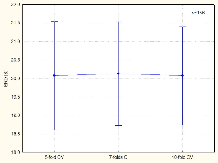
Figure 1 illustrates the bias and variance of the k-fold cross-validation.

(10)

-10-

Figure 1. k-Fold cross validation exhibits the same bias for different value of k. Error bars correspond to 95 % confidence intervals. Levene's test suggest the homogeneity of variances (p=0.289). The variance is somewhat lower as the number k increases, but it is not significant.

--- Figure 1 should be placed around here ---

However, the biases are unambiguously different in Factor 3 and the categorization of classifiers is possible.

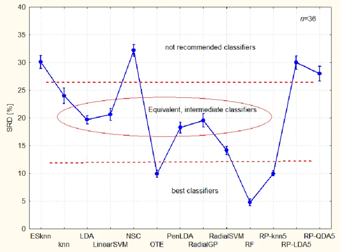
The confidence interval has been calculated from 36 objects (data set & arrangements). The variances are not homogeneous here, as expected. It is relatively easy to divide the classifiers into three groups (visually):

(11)

-11-

Figure 2. Categorization of classifiers (best ones have the smallest bias and smallest variance alike). The dotted lines are arbitrary thresholds, visually set. Abbreviations: RP – random projection²⁰; the number after the abbreviations means “Sufficient Dimension Reduction assumption” SDR5; LDA– linear discriminant analysis; QDA – quadratic discriminant analysis;

knn – k-nearest neighbors; RF – Random Forest²¹; SVM – Support Vector Machine²²; GP – Gaussian process²³; PenLDA – Penalized LDA²⁴; NSC – Nearest Shrunken Centroids²⁵; OTE – Optimal Tree Ensemble²⁶; ESknn – Ensemble of Subset of k-nearest-neighbor classifiers²⁷. Linear- and radial basis function has also been used with GP and SVM, linear and radial respectively. Numbers after the abbreviations mean the training set of size of n (a subsample of the data, and then the remaining data formed the test set.

The best classifiers (closest to the hypothetical best one) are random forest, optimal tree ensembles, and the random-projection ensemble k-nearest neighbor classifier.

(12)

-12-

Almost all classifiers are significantly different, however post hoc tests (Bonferroni and Scheffé) amalgamate four of them (LDA, LinearSVM, PenLDA and Radial GP). Indeed, they are related techniques; it shows the inner consistency of the SRD analysis. Classifiers between SRD values of 18 and 21 are in the medium group, while the weakest ones have SRD values greater than 25.

Not recommended classifiers are as follows: nearest shrunken centroids, ensemble of subset of k-nearest-neighbor classifier, and RP-LDA5 and RP-QDA5. Interestingly, the latter two, low dimensional random projections of the data have higher bias and higher variance than their counterpart, RP-knn5.

It is interesting to mention that random projection to optimal dimension is not necessarily a viable option; it can provide low bias and small variance and reversely high bias and high(er) variance. The reason is probably that the optimized solution can hardly be further improved; on the other hand, not perfect technique(s) such as knn can be significantly improved by random projection.

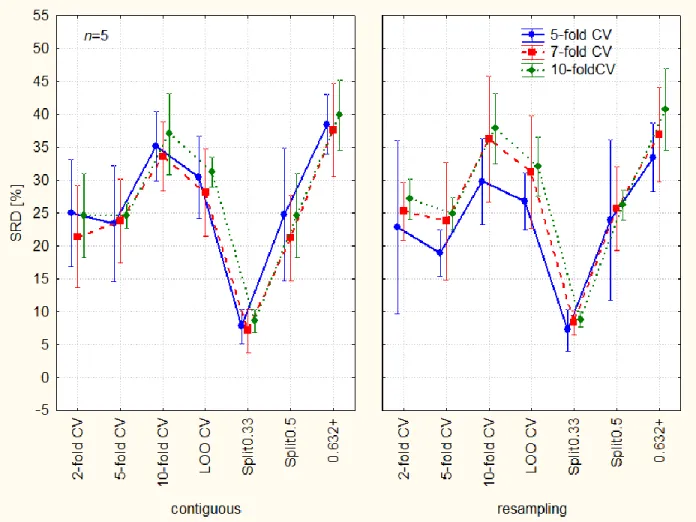
ANOVA makes the investigation of interaction terms (coupling) possible. A very specific pattern arises when one surveys Figure 3. The variance decreases as the number of fold increases, but only in case of stratified contiguous sampling. The repeated resampling destroys this pattern.

(13)

-13-

Figure 3. Interaction of the three factors: ways of cross-validation (validation variants): stratified, i.e. contiguous, A) and (Monte Carlo) resampling, B). Line plots show the number of folds (5, 7, and 10), blue solid line (5), red dashed line (7), and green pointed line (10). The abbreviations are resolved at Figure 2.

This fact emphasizes that the original data sets were not randomly processed. A definite data structure is revealed. The performance of each classifier has been studied under the influence of the number of objects in increasing order: 50, 200, 1000; 50, 100, 200; etc. Naturally this structure disappears in case of repeated random selection of the left out part for the SRD analysis. Hence, we think, it is not an artefact but a new way to discover hidden structure in the data. SRD coupled with ANOVA is so sensitive that it can detect even subtle differences.

3.2 Case study number 2. Comparison of resampling methods

The resampling methods and cross-validation are used as synonyms in the literature: In the absence of a large set of independent validation data, “a common approach to estimating predictive accuracy is based on some form of resampling the original data, e.g. cross-validation”.²⁸ These techniques divide the data into training and test sets, and range in complexity from the popular training-test split to k-fold cross-validation, Monte-Carlo k-fold cross-validation and bootstrap resampling. The original authors of ref.²⁸ used these resampling methods for model building and prediction error estimation alike: They “have performed extensive comparison of resampling methods to estimate prediction error using simulated (large signal-to-noise ratio), microarray (intermediate signal to noise ratio) and proteomic data (low signal-to-noise ratio), encompassing increasing sample sizes with large numbers of features. The impact of feature selection on the performance of various cross-validation methods is highlighted.” To make a clear distinction between their cross-validation types and ours, the former will be called resampling methods and the latter as validation variants, further on.

Again, the row minimum has been selected as a gold standard for SRD calculations being a natural choice of data fusion step. It is equivalent with the assumption of the hypothetical “best”

resampling method, which provides the most efficient estimation of the prediction error for each data table. (Transpose of tables 2 and 3 in the original publication.²⁸). Most efficient estimation means the smallest variance. SRD values were calculated for all three factors; the number of Monte Carlo repetitions (folds) was the same as the repetitions for stratified sampling to achieve balanced

(14)

-14-

and comparable results. Altogether 210 SRD values were calculated. The results of variance analysis can be seen in Table 2.

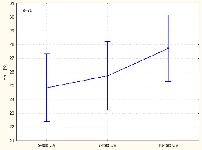
The constant term (intercept), the k-fold CV (F2), resampling methods (F3), and their interaction (F2*F3) are significant at the 5 % level. The bias increases as the number of fold increases (see Figure 4) “smaller training set produce bigger prediction errors”.²⁹ Although the theoretical deductions are not always found in case of empirical examinations, to find such a trend is surprising and reassuring.

Figure 4 illustrates the bias and variance of the k-fold cross-validation (factor 2, F2).

(15)

-15-

Figure 4. k-Fold cross-validation exhibits increasing bias as the number of fold increases. Error bars correspond to 95 % confidence interval. Levene's test suggest the homogeneity of variances (p=0.755).

The biases are unambiguously different in Factor 3 and the categorization of resampling methods is possible.

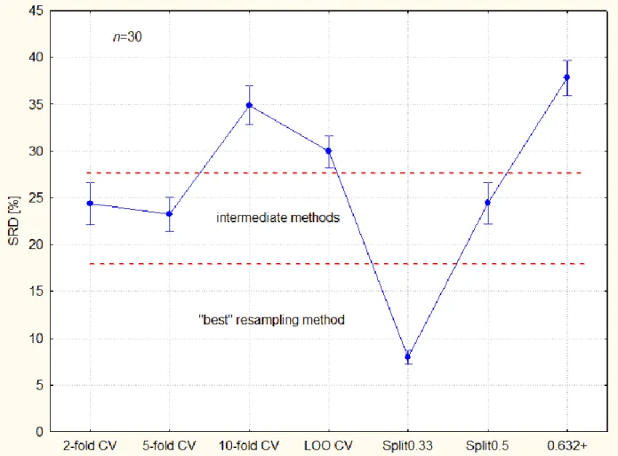
The confidence interval has been calculated from 30 objects (various data sets & changing number of objects). According to the expectances the variances are not homogeneous, either. It is relatively easy to divide the resampling methods into three groups (visually):

(16)

-16-

Figure 5. Categorization of resampling methods published in ref.²⁸ validation variants (the best one has the smallest bias and smallest variance alike). The dotted lines are arbitrary thresholds, visually set. Abbreviations: Split0.33 and split0.5. – split sample, also known as the learning-test split or holdout method, a split of training and test sets 2/3-1/3 and 1/2-1/2, respectively; 2-fold CV, 5-fold CV and 10-fold CV – k-fold cross validation k = 2, 5, and 10, respectively; LOO CV – leave-one-out cross-validation; and .632+ – corrected bootstrap.

The distinct role of Split0.33 is illustrated well and it supports the common technique of 2/3- 1/3 split in external validation.

Based on the Bonferroni and Scheffé post-hoc tests, three resampling methods belong together:

2-fold-, 5-fold CV and Split0.5 are not significantly different, but all others are from them and from each other. This fact can be explained by their close resemblance. The bootstrap estimation has the largest bias, which is understandable because of probable overcorrection for the highly unbalanced data sets. There are indications that leave-one-out bootstrap error” closely agrees with half-sample cross-validation (where x is repeatedly split into equal sized training and test sets)”.²⁹

The interaction terms (coupling) of the three factors has also been investigated with ANOVA.

A very specific pattern arises when one surveys Figure 6. The bias increases as the number of fold increases, but only in case of resampling (B): No crossings of the lines can be observed in Figure 6B. No exception exists: the rule is blue < red < green in Figure 6B. The stratified contiguous sampling destroys this pattern.

(17)

-17-

Figure 6. Interaction of the three factors: ways of cross-validation (validation variants): F1–

stratified, i.e. contiguous, A) and F2–(Monte Carlo) resampling, B). Line plots show the number of folds (5, 7, and 10), blue solid line (5), red dashed line (7), and green pointed line (10).

(F3–resampling methods by Molinari et al.’s.²⁸) The original data matrix of Case Study 2 has 15 rows, that’s why here in case of 10-fold CV, the results of A and B type CVs (green pointed lines) are equal to leave-one-out and bootstrap CV. The resampling methods are located on the x axes;

their abbreviations are explained in the title of Figure 5.

This observation stresses the possibility of preserving (or forming) systematic patterns in the data even after repeated random sampling.

3.3 Comparison of models predicting retention indices: Case study number 3

We have gathered numerous models^30-33 for prediction of retention indices of polycyclic aromatic hydrocarbons in the so-called Lee’s scale. Herewith, the row average has been selected as a gold standard for SRD calculations being a natural choice of data fusion step. It corresponds

(18)

-18-

to the maximum likelihood principle, also called as consensus ranking. The random- and systematic errors of models cancel each other out. The input table can be found in supplementary material (Table S3). SRD values were calculated for all three factors; the number of Monte Carlo repetitions (folds) was the same as the repetitions for stratified sampling to achieve balanced and comparable results. Altogether 1500 SRD values were calculated. The results of variance analysis can be seen in Table 3.

The constant term (intercept), and all the three factors and the interaction term of F1 and F2 are significant at the 5 % level. The significance of factors is understandable because of the large number of objects involved. The bias drops between 5- and 7-fold CV (see Figure 7) whereas the variance remains constant.

(19)

-19-

Figure 7. k-Fold cross validation exhibits a bias drop as the number of fold increases. Error bars correspond to 95 % confidence interval. Levene's test suggest the homogeneity of variances (p = 0.0587).

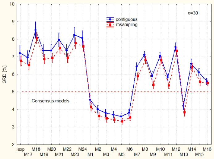
A characteristic pattern can be seen between resampling methods on the interaction plots of the F1 and F3 factors.

Monte Carlo resampling produces smaller bias, systematically for all models without exception.

All models can be categorized easily: consensus models are the best ones: M1-M6 and M13;

whereas experimental data distributes the models into acceptable and inacceptable ones. Models with larger SRD values than SRD for Iexp rationalize the information worse than the experimental data themselves (e.g. in table form). Not recommended models are as follows in order of increasing SRD values: M19 M20 M22 M12 M21 M24 M23 M18.

(20)

-20-

Figure 8. Interaction of way of cross-validation (F1) and models (F3). Error bars correspond to 95 % confidence interval. Levene's test suggest the inhomogeneity of variances (p= 0.0000).

Models denoted by M17-M24 stem from ref.³², M1-M6 from ref.³⁰, and the remaining ones from ref.³¹

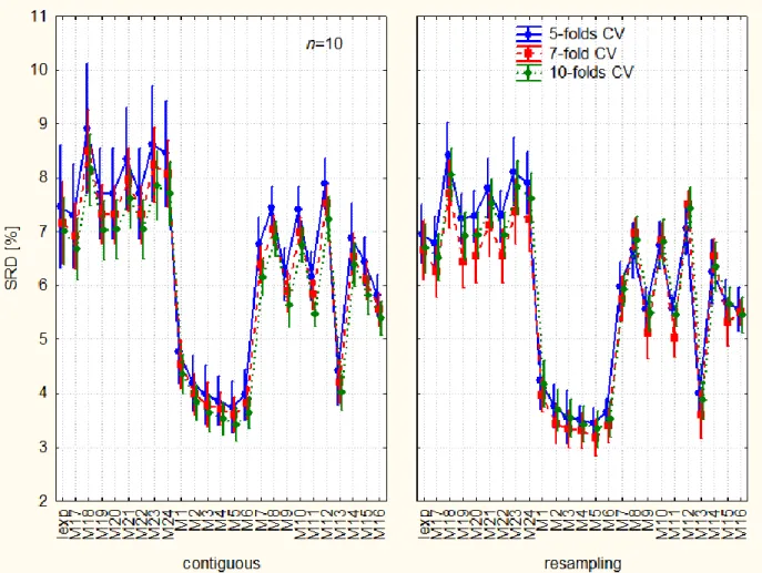
Even better decomposition can be observed in the interaction plot of three factors (Figure 9).The overlapping points and error bars might be disturbing, still the pattern is unambiguous: for contiguous blocks the bias decreases as the number of fold increases: 5, 7, and 10 without exception, whereas for resampling the ordering is not unambiguous, but mainly 5, 10, and 7. This fact, again highlights the facts that SRD with ANOVA is able to detect subtle differences if some order exists in the data structure of the input matrix.

However, the significance and pattern in validation variants is not an inherent feature of F1 and F2 factors, as it is proven by the lost significance for them if we randomize (permute) the rows of the input matrix. The details are shown in supplementary material no 2.

(21)

-21-

Figure 9. Interaction of the three factors: ways of cross-validation: stratified, i.e. contiguous, A) and (Monte Carlo) resampling, B). Line plots show the number of folds (5, 7, and 10), blue solid line (5), red dashed line (7), and green pointed line (10). The notation for models are plotted on the x axes.

3.4 Individual conclusions for case studies 1-3.

Case study no. 1 Largest variance was found for contiguous block and 5-fold cross- validation. The bias (SRD) is the same: 5-7-10 folds CV. The hypothetically best classifiers are approximated by random forest, RF, random projection-knn5 and penalized-LDA; which give the smallest bias, as well. Smallest variance was found for RP-knn5, RF, OTE. Not recommended classifiers are (the worst ones): NSC, Esknn, RP-LDA5, RP-QDA5

Case study no. 2. The bias (i.e. the SRD) increases as the number of fold increases in the order of 5-<7-< 10 folds CV. The data of Molinari et al. suggest that the best validation variant is

(22)

-22-

the 2/3 - 1/3 split. Several validation variants are equivalent: 2-, and 5-fold CV and split-1/2 are intermediate, whereas bootstrap 0.632+ proved to be the worst option.

Case study no. 3. The bias and the variance were larger for 5-fold CV; and especially contiguous block exhibited larger bias. Experimental values split the models into acceptable (“good”) and not recommended (“bad”) ones. The consensus models are the best and some of them are equivalent.

4. CONCLUSION

Sum of (absolute) ranking differences coupled with analysis of variance provides a unique measures for grouping and ordering. SRD can be considered a sensitive measure for bias and is validated by a permutation (randomization) test. Its variance can be ascertained by cross- validation: stratified contiguous blocks and/or repeated (Monte Carlo) resampling.

There is no beatific way of cross-validation, which is always better independently from the data structure. No validation variant is superior in all circumstances. As the number of folds in k- fold cross-validation increases, the variance decreases, as expected, especially in case of the contiguous (stratified) sampling, c.f. figure 3. Less bias can be observed for resampling than in case of contiguous sampling; however, it can be advantageous for a conservative estimation (c.f.

Figure 8). In case of large number of compared items, the same variance decrease can be observed for contiguous sampling plus the bias also decreases in the same manner (solid line, dashed line, dotted line in Figure 9.) However sevenfold cross-validation has less bias for repeated (Monte Carlo) resampling. The optimal validation variant should be determined individually again and again.

However, the way of validation does not exert a significant effect on ANOVA of SRD values, provided that no systematic structure is present in the data. Other way around, SRD is sensitive enough to reveal the non-negligible structure in the data. In any case, a randomization of objects (samples) is recommended before any SRD analysis.

Independently of the various and “adjustable” effect of validation variants on the results the SRD could find subtle differences in this case, as well, similarly to the earlier experience.³⁴

(23)

-23- ACKNOWLEDGEMENT

The work was supported by the National Research, Development and Innovation Office of Hungary under grant numbers OTKA K 119269 and KH_17 125608.

REFERENCES

1. Rücker C, Rücker G, Meringer M. y-Randomization and Its Variants in QSPR/QSAR, J Chem Inf Model. 2007;47:2345-2357. https://doi.org/10.1021/ci700157b

2. Miller, A. Subset selection in regression. Part 1.4 ‘Black box’ use of best-subset selection techniques, London: Chapman and Hall; pp. 13 (1990).

3. Gramatica P. External Evaluation of QSAR Models, in Addition to Cross- Validation:

Verification of Predictive Capability on Totally New Chemicals. Mol Inf. 2014;33(4):311- 314. https://doi.org/10.1002/minf.201400030

4. Gramatica P. Principles of QSAR models validation: internal and external. QSAR Comb Sci. 2007;26(5):694-701. https://doi.org/10.1002/qsar.200610151

5. Hastie T, Tibshirani R, & Friedman JH. Chapter 7.10 Cross-Validation in: The elements of statistical learning: Data mining, inference, and prediction. 2nd ed., pp. 241-249). New York: Springer; 2009.

6. Gütlein M, Helma C, Karwath A, & Kramer S. A large-scale empirical evaluation of cross- validation and external test set validation in (Q)SAR. Mol Inf. 2013;32(9-10):516-528.

https://doi.org/10.1002/minf.201200134

7. Kohavi R. A Study of Cross-Validation and Bootstrap for Accuracy Prediction and Model Selection, IJCAI'95 Proceedings of the 14th International Joint Conference on Artificial Intelligence Volume 2, Pages 1137-1143 Montreal, Quebec, Canada—August 20-25, 1995.

8. http://wiki.eigenvector.com/index.php?title=Using_Cross-Validation accessed at March 23 / 2018.

9. Héberger K. Sum of ranking differences compares methods or models fairly. TrAC–Trends Anal Chem. 2010;29(1):101‐109. https://doi.org/10.1016/j.trac.2009.09.009

10. Héberger K, Kollár‐Hunek K. Sum of ranking differences for method discrimination and its validation: comparison of ranks with random numbers. J Chemom. 2011;25(4):151‐158.

(24)

-24-

11. Bin J, Ai F-F, Fan W, Zhou J-H, Yun Y-H, & Liang Y-Z. A modified random forest approach to improve multi-class classification performance of tobacco leaf grades coupled with NIR spectroscopy RSC Adv. 2016;6:30353-30361

https://doi.org/10.1039/C5RA25052H

12. Youden WJ. Statistical Manual of the Association of Official Analytical Chemists.

Statistical techniques for collaborative test, 8^th Edition., AOAC International, Gaithersburg, MD, USA, 1997 pp. 1-63.

13. Willett P. Combination of similarity rankings using data fusion. J Chem Inf Model.

2013;53:1-10.

14. Gramatica P, Giani, E, Papa E. Statistical external validation and consensus modeling: A QSPR case study for Koc prediction. Journal of Molecular Graphics and Modelling 2007;25(6):755-766.

15. Kollár-Hunek K, & Héberger K. Method and model comparison by sum of ranking differences in cases of repeated observations (ties). Chemometr Intell Lab Syst.

2013;127:139-146. https://doi.org/10.1016/j.chemolab.2013.06.007

16. Bajusz D, Rácz A, & Héberger K. Why is Tanimoto index an appropriate choice for fingerprint-based similarity calculations? J Cheminform. 2015;7: Article Number 20.

https://doi.org/10.1186/s13321-015-0069-3

17. Stokes TD, Fotein M, Brownfield B, Kalivas JH, Mousdis G, Amine A, & Georgiou C.

Feasibility Assessment of Synchronous Fluorescence Spectral Fusion by Application to Argan Oil for Adulteration Analysis. Appl Spectr. 2018;72(3):432-441.

https://doi.org/10.1177/0003702817749232

18. Sipos L, Gere A, Popp J, Kovács S. A novel ranking distance measure combining Cayley and Spearman footrule metrics. J Chemom. 2018;32:e3011.

19. Lourenco J, and Lebensztajn L. Post-Pareto Optimality Analysis with Sum of Ranking Differences. IEEE Transactions on Magnetics 2018;PP(99):1-10.

https://doi.org/10.1109/TMAG.2018.2836327

20. Cannings TI, & Samworth RJ. Random-projection ensemble classification. J R Statist Soc B. 2017;79(4):959-1035. https://arxiv.org/abs/1504.04595v2

(25)

-25-

21. Breiman L. Random forests. Mach Learn. 2001;45:5-32.

https://doi.org/10.1023/A:1010933404324

22. Cortes, C. and Vapnik, V. (1995) Support-vector networks. Mach Learn. 20, 273-297.

http://dx.doi.org/10.1007/BF00994018

23. Williams CKI, & Barber D. Bayesian classification with Gaussian processes. IEEE Transactions on Pattern Analysis and Machine Intelligence. 1998;20:1342-1351.

https://doi.org/10.1109/34.735807

24. Witten DM, & Tibshirani R. Penalized classification using Fisher’s linear discriminant. J.

R. Statist. Soc. B. 2011;73:753-772. https://doi.org/10.1111/j.1467-9868.2011.00783.x 25. Tibshirani R, Hastie T, Narisimhan B., & Chu, G. Class prediction by nearest shrunken

centroids, with applications to DNA microarrays. Statist Sci. 2003;18:104-117.

https://doi.org/10.1214/ss/1056397488

26. Khan, Z., Gul, A., Mahmoud, O., Miftahuddin, M., Perperoglou, A., Adler, W. and Lausen, B. An ensemble of optimal trees for class membership probability estimation. In Analysis of Large and Complex Data: Proc Eur Conf Data Analysis, Bremen, July (eds A. Wilhelm and H. A. Kestler). Berlin: Springer 2015.https://doi.org/10.1007/978-3-319-25226-1_34 27. Gul A, Perperoglou A, Khan Z, Mahmoud O, Miftahuddin M, Adler W, & Lausen B.

Ensemble of a subset of kNN classifiers.Adv Data Anal Classif. 2016; in press pp. 1-14.

https://doi.org/10.1007/s11634-015-0227-5

28. Molinaro AM, Simon R, & Pfeiffer RM. Prediction error estimation: a comparison of resampling methods. Bioinformatics. 2005;21(15): 3301-3307.

https://doi.org/10.1093/bioinformatics/bti499

29. Efron B, Tibshirani R. Cross-validation and the bootstrap. Estimating the error rate of a prediction rule. Technical report No 477, Department of Statistics, Stanford University, May 1995.

30. Liu S, Yin C, Cai S, Li Z. Molecular structural vector description and retention index of polycyclic aromatic hydrocarbons. Chemometr Intell Lab Syst. 2002;61(1-2):3-15.

https://doi.org/10.1016/S0169-7439(01)00146-0

31. Skrbic B, Djurisic-Mladenovic N, Cvejanov J. Discrimination between linear and non- linear models for retention indices of polycyclic aromatic hydrocarbons in the so-called

(26)

-26-

Lee’s scale. Chemometr Intell Lab Syst. 2004;72(2):167-171.

https://doi.org/10.1016/j.chemolab.2004.01.011

32. Drosos JC, Viola-Rhenals M, Vivas-Reyes R. Quantitative structure–retention relationships of polycyclic aromatic hydrocarbons gas-chromatographic retention indices.

J Chromatogr A. 2010;1217(26):4411-4421.

https://doi.org/10.1016/j.chroma.2010.04.038

33. Héberger K, Škrbić B. Ranking and similarity for quantitative structure–retention relationship models in predicting Lee retention indices of polycyclic aromatic hydrocarbons. Anal Chim Acta. 2012;716:92-100.

https://doi.org/10.1016/j.aca.2011.11.061

34. Andrić F, Bajusz D, Rácz A, Šegan S, Héberger K, Multivariate assessment of lipophilicity scales - computational and reversed phase thin-layer chromatographic indices, J Pharm and Biomed Anal. 2016;127:81-93. http://dx.doi.org/10.1016/j.jpba.2016.04.001

Table 1. Decomposition of validation variants and performance of classifiers, i.e. Univariate tests of significance for SRD [%]. Sigma-restricted parameterization.

SS n MS F p

Intercept 188897.6 1 188897.6 18490.55 0.000000 F1: contiguous/resampling 4.0 1 4.0 0.40 0.529743 F2: 5-, 7- and 10-fold CV 0.3 2 0.2 0.02 0.984672 F3: Classifier 32405.8 12 2700.5 264.34 0.000000

F1*F2 4.2 2 2.1 0.21 0.814220

F1*F3 23.0 12 1.9 0.19 0.998851

F2*F3 43.9 24 1.8 0.18 0.999996

F1*F2*F3 64.2 24 2.7 0.26 0.999869

Error 3984.2 390 10.2

Factors: F1 – way of cross validation (validation variantsvarainats), two levels: contiguous and resampling; F2 – number of folds, three levels: 5-, 7- and 10-fold cross-validation, and F3 – classifiers to be compared, (13 levels, see supplementary material 1 for details). Abbreviations: SS – sum of squared residuals; n – degree of freedom; MS – mean squared residuals, F – Fisher criterion; p – probability of significance.

(27)

-27-

Table 2. Decomposition of cross-validation variants and resampling methods, i.e. Univariate tests of significance for SRD [%]. Sigma-restricted parameterization.

SS n MS F p

Intercept 143137.3 1 143137.3 5559.096 0.000000 F1: contiguous/resampling 0.0 1 0.0 0.001 0.974257 F2: 5-, 7- and 10-fold CV 304.1 2 152.1 5.906 0.003321 F3: resampling methods 17142.8 6 2857.1 110.964 0.000000

F1*F2 265.2 2 132.6 5.149 0.006754

F1*F3 76.4 6 12.7 0.495 0.811657

F2*F3 96.2 12 8.0 0.311 0.986700

F1*F2*F3 49.5 12 4.1 0.160 0.999453

Error 4325.7 168 25.7

F3 – resampling methods to be compared, seven levels. Explanations for all other notations and abbreviations can be found at Table 1.

Table 3. Decomposition of validation variants and resampling methods, i.e. Univariate tests of significance for SRD [%]. Sigma-restricted parameterization.

SS n MS F p

Intercept 54040.93 1 54040.93 111398.9 0.000000 F1: Contiguous/resampling 55.53 1 55.53 114.5 0.000000 F2: 5-, 7- and 10-fold CV 37.31 2 18.65 38.5 0.000000 F3: Models 3633.41 24 151.39 312.1 0.000000

F1*F2 16.49 2 8.24 17.0 0.000000

F1*F3 5.20 24 0.22 0.4 0.990556

F2*F3 9.44 48 0.20 0.4 0.999908

F1*F2*F3 8.94 48 0.19 0.4 0.999959

Error 654.90 1350 0.49

F3–models for predicting retention indices to be compared, 25 levels. Explanations for all other notations and abbreviations can be found at Table 1.

(28)

-28- Figure captions:

Figure 1. k-Fold cross validation exhibits the same bias for different value of k. Error bars correspond to 95 % confidence intervals. Levene's test suggest the homogeneity of variances (p=0.289). The variance is somewhat lower as the number k increases, but it is not significant.

Figure 2. Categorization of classifiers (best ones have the smallest bias and smallest variance alike). The dotted lines are arbitrary thresholds, visually set. Abbreviations: RP – random projection²⁰; the number after the abbreviations means “Sufficient Dimension Reduction assumption” SDR5; LDA– linear discriminant analysis; QDA – quadratic discriminant analysis;

knn – k-nearest neighbors; RF – Random Forest²¹; SVM – Support Vector Machine²²; GP – Gaussian process²³; PenLDA – Penalized LDA²⁴; NSC – Nearest Shrunken Centroids²⁵; OTE – Optimal Tree Ensemble²⁶; ESknn – Ensemble of Subset of k-nearest-neighbor classifiers²⁷. Linear- and radial basis function has also been used with GP and SVM, linear and radial respectively. Numbers after the abbreviations mean the training set of size of n (a subsample of the data, and then the remaining data formed the test set.

Figure 3. Interaction of the three factors: ways of cross-validation (validation variants): stratified, i.e. contiguous, A) and (Monte Carlo) resampling, B). Line plots show the number of folds (5, 7, and 10), blue solid line (5), red dashed line (7), and green pointed line (10). The abbreviations are resolved at Figure 2.

Figure 4. k-Fold cross validation exhibits increasing bias as the number of folds increases. Error bars correspond to 95 % confidence interval. Levene's test suggest the homogeneity of variances (p=0.755).

Figure 5. Categorization of resampling methods published in ref.²⁸ (the best one has the smallest bias and smallest variance alike). The dotted lines are arbitrary thresholds, visually set.

Abbreviations: Split0.33 and split0.5. – split sample, also known as the learning-test split or holdout method, a split of training and test sets 2/3-1/3 and 1/2-1/2, respectively; 2-fold CV, 5- fold CV and 10-fold CV – k-fold cross validation k = 2, 5, and 10, respectively; LOO CV – leave- one-out cross-validation; and .632+ – corrected bootstrap.

Figure 6. Interaction of the three factors: ways of cross-validation (validation variants): F1–

stratified, i.e. contiguous, A) and F2–(Monte Carlo) resampling, B). Line plots show the number

(29)

-29-

of folds (5, 7, and 10), blue solid line (5), red dashed line (7), and green pointed line (10).

(F3–resampling methods by Molinari et al.’s.²⁸) The original data matrix of Case Study 2 has 15 rows, that’s why here in case of 10-fold CV, the results of A and B type CVs (green pointed lines) are equal to leave-one-out and bootstrap CV. The resampling methods are located on the x axes;

their abbreviations are explained in the title of Figure 5.

Figure 7. k-Fold cross validation exhibits a bias drop as the number of folds increases. Error bars correspond to 95 % confidence interval. Levene's test suggest the homogeneity of variances (p=

0.0587).

Figure 8. Interaction of way of cross-validation (F1) and models (F3). Error bars correspond to 95 % confidence interval. Levene's test suggest the inhomogeneity of variances (p= 0.0000).

Models denoted by M17-M24 stem from ref.³², M1-M6 from ref.³⁰, and the remaining ones from ref.³¹

Figure 9. Interaction of the three factors: ways of cross-validation: stratified, i.e. contiguous, A) and (Monte Carlo) resampling, B). Line plots show the number of folds (5, 7, and 10), blue solid line (5), red dashed line (7), and green pointed line (10). The notations for models are plotted on the x axes.