(2006) pp. 3–13
http://www.ektf.hu/tanszek/matematika/ami
Multiple root finder algorithm for Legendre and Chebyshev polynomials via Newton’s
method
Victor Barrera-Figueroa
a, Jorge Sosa-Pedroza
b, José López-Bonilla
ca b c
Instituto Politécnico Nacional, Escuela Superior de Ingeniería Mecánica y Eléctrica, Sección de Estudios de Postgrado e Investigación
ae-mail: vbarreraf@ipn.mx;be-mail:jsosa@ipn.mx;ce-mail:jlopezb@ipn.mx
Submitted 23 June 2006; Accepted 31 October 2006
Abstract
We exhibit a numerical technique based on Newton’s method for finding all the roots of Legendre and Chebyshev polynomials, which execute less itera- tions than the standard Newton’s method and whose results can be compared with those for Chebyshev polynomials roots, for which exists a well known analytical formula. Our algorithm guarantees at least nine decimal correct ciphers in the worst case, however, when comparing with Chebyshev roots given by its formula, even eighteen decimal correct ciphers are achieved in several roots, in the best case. As a comparison guide the results are collated with those gotten by MATLAB.
Keywords: Newton’s method, Legendre polynomials, Chebyshev polynomi- als, multiple root finder algorithm.
1. Introduction
Legendre polynomials (see [1, 2, 3, 4]) as well as Chebyshev (see [1, 2, 3, 4, 5]) ones has found countless applications in all branches of engineering and sci- ence, among which the most representatives include calculation of quadratures, electromagnetics and antenna applications, solutions for potential theory and for Schrödinger’s equation, aerodynamics and mechanics applications, etc. This is due mainly because the use of their roots allows us to solve a specific problem with the best efficiency.
These polynomials are very similar to each other, not only in the form of their respective differential equation, but also in the numerical values of their roots.
3
However, sometimes it is better the use of Legendre polynomials instead of Cheby- shev ones because by using their roots, one can reach the most optimized solution.
For instance, when calculating a quadrature, Gauss established that the best way for obtaining the minimum error in a numerical integration is by dividing the inte- gration domain in agreement with the way Legendre roots are distributed on their own domain.
So, because of the wide use of Legendre and Chebyshev roots, this paper presents a multiple root finder algorithm, which is expected to be a useful tool, not only in engineering work but also in numerical and mathematical analysis. This algorithm is based in the classical Newton’s method (see [2]), however, we have made some modifications in order to find all the roots of an specific polynomial by using the improved Newton’s method (see [2]).
2. Newton’s method
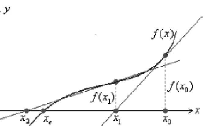
Newton’s process is a numerical tool used to find the zero xe of a real-valued functionf(x), continuously differentiable and whose derivative does not vanish at x=xe. The method consists in proposing an initial rootx0 which must be in the neighborhood ofxe, as shown in Figure 1. Once made this, we draw a tangent line tof(x)atx=x0, and determine its intersection with thexaxis. The equation for the line is:
y=f(x0) +f′(x0)(x−x0), (2.1) which means that locally, in the small neighborhood of x0,f(x)can be considered as a linear equation, even iff(x)is not linear. We should notice that this equation corresponds to the truncate Taylor series with center at x=x0 by neglecting the remainder term. The intersection, named x1, is then:
x1−x0=−f(x0)
f′(x0), (2.2)
Now,x1is closer to the real zeroxe, and it will be used to draw the next tangent line tof(x)atx=x1 which produces the intersectionx2. So, in thenthiteration, the intersection of the tangent line with thexaxis will be [2]:
xn=xn−1− f(xn−1)
f′(xn−1), n= 1,2,3, . . . (2.3) After a number of iterations xn will be close enough to xe. In this way, once we have established the allowed error ǫfor the zero, we can set the condition for stopping the method, which is reached when:
|xn−xn−1|6ǫ. (2.4)
Newton’s technique will usually converge provided the initial guess is close enough to true root. Furthermore, for a zero of multiplicity 1, the convergence
Figure 1: Tangent lines tof(x)atx=x1.
is at least quadratic in a neighborhood of xe, which intuitively means that the number of correct digits roughly at least doubles in every step.
Newton’s method acquire a bigger convergence if in Taylor series we consider the quadratic term:
y=f(x0) +f′(x0)(x−x0) +1
2f′′(x0)(x−x0)2, (2.5) that is, in the small neighborhood of x0, f(x) can be considered as a quadratic equation, even iff(x)is not quadratic. The intersection x1 between (2.5) and the xaxis can be calculated from:
x1−x0=− f(x0)
f′(x0) +12f′′(x0)(x1−x0), (2.6) by substituting (2.2) into (2.6) we get:
x1−x0=− 2f(x0)f′(x0)
2 [f′(x0)]2−f(x0)f′′(x0). (2.7) So, in thenthiteration, we have the next recursive formula (see [2]):
xn=xn−1− 2f(xn−1)f′(xn−1)
2 [f′(xn−1)]2−f(xn−1)f′′(xn−1), n= 1,2,3, . . . (2.8) This is the improved Newton’s method which converges faster than the original one. As well as we have to know the first derivative of f(x)in both methods, in the improved one, we must know the second derivative off(x)in each point. This could be a problem if f(x)is not an analytical formula but a set of data points, in which both derivatives could be calculated from standard numerical techniques.
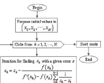
3. Multiple root finder algorithm based on Newton’s process
The application of Newton’s method to a polynomial in the quest for all its roots could be easily implemented if we express it according to the fundamental theorem of Algebra:
f(x) =k(x−x1)(x−x2). . .(x−xN), (3.1) where N is the polynomial order, k is a proportionality constant and {x1, x2, . . . , xN} are all the polynomial roots, which are not necessarily put in order. In the following, the subindexj in the rootxj represents the number of root and it should not be confused with the number of iterations used in the previous sections which will be omitted from here. By applying Newton’s algorithm to the polynomial (3.1) for searching the first rootx1, we have the next recursive relation:
x1=x1− f(x)
f′(x). (3.2)
Oncex1 is found, we built the polynomial g(x)of orderN −1 which has not x1 as one of its roots:
g(x) = f(x) x−x1
=k(x−x2)(x−x3). . .(x−xN), (3.3) and by applying Newton’s technique tog(x)we determine the next rootx2and so on. So, in thekthstep, we built the following polynomial:
g(x) = f(x) Qk−1
i=1(x−xi), (3.4)
and, according to Newton’s method, thekth root is:
xk =xk− g(xk)
g′(xk), (3.5)
which implies the calculation for the derivative ofg(x)which could not be so evident because of the need to find the derivative of the product term. Such derivative is:
d dx
k−1
Y
i=1
(x−xi) = 1
x−x1
+ 1
x−x2
+· · ·+ 1 x−xk−1
k−1
Y
i=1
(x−xi) =
=
k−1
Y
i=1
(x−xi)
k−1
X
i=1
1 x−xi
, (3.6)
therefore the derivative forg(x)is:
g′(x) = 1 Qk−1
i=1(x−xi)
"
f′(x)−f(x)
k−1
X
i=1
1 x−xi
#
. (3.7)
By substituting (3.7) and (3.4) into (3.5) we reach the recursive relation for getting all the roots for the polynomialf(x):
xk =xk− f(xk) f′(xk)−f(xk)Pk−1
i=1 1 x−xi
, k= 1,2, . . . , N. (3.8) On the basis of (3.8) we express the multiple root finder algorithm with the following diagram:
Figure 2: Multiple root finder algorithm.
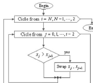
In order to sort all the roots given by the multiple root finder process, we can introduce the well known bubble sort method which by successively interchanging theN roots can provide us the list of expected results. The bubble sort method is drawn in the following diagram:
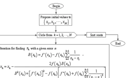
4. Multiple root finder algorithm based on improved Newton’s method
In order to improve the algorithm’s convergence, we can introduce Newton’s technique in the quest for all the polynomial roots. In first term we look at the
Figure 3: Bubble sort method for putting in order the polynomial’s roots.
rootx1 of the polynomial (3.1) with the recursive relation (2.8). Oncex1is found, we built the polynomial g(x), (3.3). By applying improved Newton’s method to g(x) we found the next root x2 and so on. So, in the kth step, we built the polynomial (3.4), from which thekthroot is:
xk=xk− 2g(xk)g′(xk)
2 [g′(xk)]2−g(xk)g′′(xk). (4.1) Iterative formula (4.1) implies the calculation for the second derivative ofg(x) which could a hard task, however, the result is not as difficult as one could expect:
g′′(x) =
f′′(x)−2f′(x)
k−1
P
i=1 1
x−xi +f(x)
"
k−1
P
i=1 1 (x−xi)2 +
k−1 P
i=1 1 x−xi
2#
k−1
Q
i=1
(x−xi)
. (4.2)
So by substituting (3.4),(3.7) and (4.2) into (4.1) we get:
xk=xk− 2f(xk)B(xk) B2(xk) + [f′(xk)]2−f(xk)
f′′(xk) +f(xk)
k−1
P
i=1 1 (xk−xi)2
, (4.3)
B(xk) =f′(xk)−f(xk)
k−1
X
i=1
1 xk−xi
, k= 1,2, . . . , N.
Notice the similarity between (4.1) and (4.3) where f(xk) is similar to g(xk), and g′(xk) is analogous to B(xk). Obviously both formulas are not completely analogous, but the existent similarity is notorious. On the basis of (4.3) we express the improved multiple root finder algorithm with the following diagram, Figure 4, again, the bubble sort method could be used in order to sort the obtained roots:
Figure 4: Improved multiple root finder algorithm.
5. Legendre and Chebyshev polynomials roots cal- culation
In this section we present the results reached by both algorithms applied to Legendre and Chebyshev polynomials; also, it is shown the number of performed iteration. Such results are compared with those gotten by MATLAB. In the case of Chebyshev’s roots, we provide the analytical results gotten by the formula [2]:
xk= cos
2k−1 2N π
, k= 1,2, . . . , N, (5.1) whereN is the polynomial degree. Legendre polynomialsPn(x)are the solution of the Legendre differential equation:
(1−x2)d2Pn(x)
dx2 −2xdPn(x)
dx +n(n+ 1)Pn(x) = 0, n= 0,1,2, . . . , (5.2)
while Chebyshev polynomialsTn(x)are the solution for its respective differential equation:
(1−x2)d2Tn(x)
dx2 −xdTn(x)
dx +n2Tn(x) = 0, n= 0,1,2, . . . . (5.3) Both Pn(x)and Tn(x)can be defined by mean of recursive relations, which is an important issue in the numerical point of view. For Legendre polynomials, the recursive relations are:
P0(x) = 1, P1(x) =x, Pn+2=2n+ 3
n+ 2 xPn+1−n+ 1
n+ 2Pn, n= 0,1,2, . . . , (5.4) while for Chebyshev polynomials the recursive relations are:
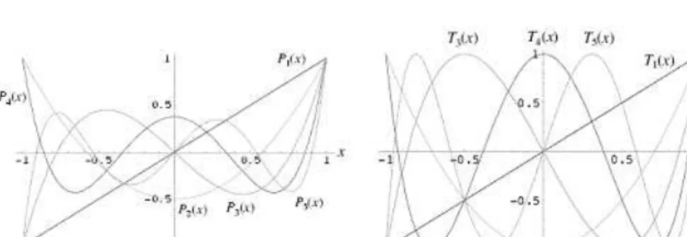
T0(x) = 1, T1(x) =x, Tn+2= 2xTn+1−Tn, n= 0,1,2, . . . , (5.5) Such polynomials are plotted in Figure 5. It is notable how the roots are clustered in the ends of the domain [−1,1]in both polynomials.
Figure 5: Legendre and Chebyshev polynomials.
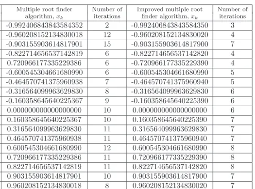
In Table 1 are shown the results forP19(x) roots reached by both algorithms, with a permissible error ofǫ= 1×10⁻¹² for each of them.
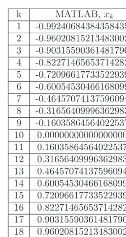
In Table 2 the roots for P19(x) obtained using MATLAB are presented for comparison. In Table 3 are shown the results for T19(x) roots reached by both algorithms, with a permissible error ofǫ= 1×10⁻¹² for each of them.
In Table 4 the roots forT19(x)obtained using (5.1) and MATLAB are presented for comparison.
6. Conclusions
Both algorithms have shown to be effective in finding all the roots for a specific polynomial. Such polynomial must have all its roots real and with simple mul- tiplicity. These conditions are satisfied by Legendre and Chebyshev polynomials.
Multiple root finder Number of Improved multiple root Number of
k algorithm,xk iterations finder algorithm,xk iterations
1 -0.992406843843584352 2 -0.992406843843584350 3 2 -0.960208152134830018 12 -0.960208152134830020 4 3 -0.903155903614817901 15 -0.903155903614817900 7 4 -0.822714656537142819 6 -0.822714656537142820 4 5 0.720966177335229386 6 -0.720966177335229390 4 6 -0.600545304661680990 6 -0.600545304661680990 5 7 -0.464570741375960938 7 -0.464570741375960940 5 8 -0.316564099963629830 8 -0.316564099963629830 6 9 -0.160358645640225367 9 -0.160358645640225390 6 10 0.000000000000000000 10 0.000000000000000000 6 11 0.160358645640225367 10 0.160358645640225390 7 12 0.316564099963629830 11 0.316564099963629830 7 13 0.464570741375960938 11 0.464570741375960940 7 14 0.600545304661680990 12 0.600545304661680990 8 15 0.720966177335229386 11 0.720966177335229390 8 16 0.822714656537142819 11 0.822714656537142820 8 17 0.903155903614817901 10 0.903155903614817900 7 18 0.960208152134830018 8 0.960208152134830020 7 19 0.992406843843584352 8 0.992406843843584460 5
Table 1: Roots forP19(x)with both algorithms.
However, for other type of polynomials, another process is being developed in order to get not only their real roots but also their complex ones, taking into account their own multiplicity.
The first algorithm is faster than the second one, because it performs fewer operations than the improved one, which must calculate the second derivative and several sums, among other operations. However, the second algorithm executes less iteration than the first one, and this fact could be useful in finding the roots for polynomials of big order. Both algorithms provide us several correct ciphers when comparing with the results gotten by MATLAB, however, both are faster than the routines used by MATLAB in doing the same action.
It is expected that these algorithms can be employed as a part for several programs which must involve quadratures or interpolations (among other numerical issues) while looking for engineering or science solutions, because of its speed and ease for programming. We the authors recommend an error of ǫ= 1×10⁻¹² for each root, which has shown to provide correct results for all the possible polynomial degrees. However, for an error of ǫ= 1×10⁻¹⁸ in some degrees, both algorithms perform a great number of iterations in which the loop becomes endless.
k MATLAB,xk
1 -0.992406843843584350 2 -0.960208152134830020 3 -0.903155903614817900 4 -0.822714656537142820 5 -0.720966177335229390 6 -0.600545304661680990 7 -0.464570741375960940 8 -0.316564099963629830 9 -0.160358645640225370 10 0.000000000000000000 11 0.160358645640225370 12 0.316564099963629830 13 0.464570741375960940 14 0.600545304661680990 15 0.720966177335229390 16 0.822714656537142820 17 0.903155903614817900 18 0.960208152134830020 19 0.992406843843584350 Table 2: Roots forP19(x)with MATLAB.
Multiple root finder Number of Improved multiple root Number of
k algorithm,xk iterations finder algorithm,xk iterations
1 -0.996584493006669847 2 -0.996584493006669850 3 2 -0.969400265939330374 12 -0.969400265939330370 5 3 -0.915773326655057396 15 -0.915773326655057400 7 4 -0.837166478262528546 4 -0.837166478262528550 4 5 -0.735723910673131587 5 -0.735723910673131590 4 6 -0.614212712689667817 6 -0.614212712689667820 4 7 -0.475947393037073563 7 -0.475947393037073560 5 8 -0.324699469204683511 8 -0.324699469204683510 5 9 -0.164594590280733893 9 -0.164594590280733890 6 10 0.000000000000000000 10 0.000000000000000000 6 11 0.164594590280733893 10 0.164594590280733890 7 12 0.324699469204683511 11 0.324699469204683460 7 13 0.475947393037073563 11 0.475947393037073560 7 14 0.614212712689667817 12 0.614212712689667820 8 15 0.735723910673131587 12 0.735723910673131590 8 16 0.837166478262528546 11 0.837166478262528550 8 17 0.915773326655057396 10 0.915773326655057400 7 18 0.969400265939330374 8 0.969400265939330370 7 19 0.996584493006669847 8 0.996584493006669850 5
Table 3: Roots forT19(x)with both algorithms.
Analytical formula:
k xk = cos 2k2N−1π
MATLAB,xk
1 -0.996584493006669847 -0.996584493006669850 2 0.969400265939330486 -0.969400265939330370 3 -0.915773326655057507 -0.915773326655057510 4 -0.837166478262528546 -0.837166478262528550 5 -0.735723910673131587 -0.735723910673131590 6 -0.614212712689667817 -0.614212712689667820 7 -0.475947393037073563 -0.475947393037073560 8 -0.324699469204683455 -0.324699469204683460 9 -0.164594590280733838 -0.164594590280734060 10 0.000000000000000061 0.000000000000000061 11 0.164594590280733977 0.164594590280733980 12 0.324699469204683566 0.324699469204683570 13 0.475947393037073618 0.475947393037073620 14 0.614212712689667817 0.614212712689667820 15 0.735723910673131698 0.735723910673131590 16 0.837166478262528657 0.837166478262528550 17 0.915773326655057396 0.915773326655057400 18 0.969400265939330374 0.969400265939330370 19 0.996584493006669847 0.996584493006669850 Table 4: Roots forT19(x)with analytical formula and MATLAB.
References
[1] M. Abramowitz and I. A. Stegun,Handbook of mathematical functions, Wiley and Sons, N. Y. (1972).
[2] C. Lanczos,Applied analysis, Dover N. Y. (1988).
[3] J. B. Seaborn,Hypergeometric functions and their applications, Springer-Verlag (1991).
[4] C. Lanczos, Linear differential operators, Dover N. Y. (1997).
[5] J. C. Mason and D. C. Handscomb, Chebyshev polynomials, Chapman&Hall - CRC Press (2002).
V. Barrera-Figueroa, J. Sosa-Pedroza, J. López-Bonilla UPALM. Edif. Z-4, 3er. piso, col. Lindavista, C.P. 07738, México D.F.