Volumetric flow rate reconstruction in great vessels

Volumetric flow rate reconstruction in great vessels ^*

Attila Lovas

, Róbert Nagy

, Péter Sótonyi

, Brigitta Szilágyi

aBudapest University of Technology and Economics Department of Analysis,

attila.lovas@gmail.com

bBudapest University of Technology and Economics Department of Structural Mechanics

nagy.robert@epito.bme.hu

cSemmelweis University, Department of Vascular Surgery sotonyi.peter@varosmajor.sote.hu

dBudapest University of Technology and Economics Department of Geometry

szilagyibr@gmail.com Submitted: November 12, 2018

Accepted: February 11, 2019 Published online: February 27, 2019

Abstract

We present a new algorithm to reconstruct the volumetric flux in the aorta. We study a simple 1D blood flow model without viscosity term and sophisticated material model. Using the continuity law, we could reduce the original inverse problem related to a system of PDEs to a parameter iden- tification problem involving a Riccati-type ODE with periodic coefficients.

We implemented a block-based optimization algorithm to recover the model

*This research was supported by the Higher Education Excellence Program of the Ministry of Human Capacities in the frame of Biotechnology research area of Budapest University of Technology and Economics (BME FIKP-BIO).

†The first author was also supperted by the Lendület grant LP 2015-6 of the Hungarian Academy of Sciences.

50(2019) pp. 117–130

doi: 10.33039/ami.2019.02.002 http://ami.uni-eszterhazy.hu

117

parameters. We tested our method on real data obtained using CG-gated CT angiography imaging of the aorta. Local flow rate was calculated in 10 cm long aorta segments which are located 1 cm below the heart. The reconstructed volumetric flux shows a realistic wave-like behavior, where reflections from ar- teria iliaca can also be observed. Our approach is suitable for estimating the main characteristics of pulsatile flow in the aorta and thereby contributing to a more accurate description of several cardiovascular lesions.

Keywords: Haemodynamics, pulse wave propagation, one-dimensional mod- eling, periodic Ricatti equation

MSC:92C50, 92C10, 92C35, 76B99

1. Introduction

Pulsatile flow in blood vessels has been studied for more than 300 years. Euler initiated the theory of pressure wave propagation in the vascular system in 1775 [6]. The first modern mathematical model of pulsatile flow in blood vessels was developed by Korteweg and Lamb [10, 12]. It is widely accepted that, flow wave- form carries valuable information about the physical properties of the circulatory system [1]. Moreover, it allows to calculate patient-specific estimates of haemod- inamical quantities like blood pressure in the aorta that are difficult to measure non-invasively. Consequently, haemodynamical simulations have become increas- ingly popular in the last few decades. Blood flow modeling techniques can be divided into three main types: 0D or lumped parameter models, 1D and 3D mod- els. Each of these has its own advantages and limitations. For example, 0D models are computationally inexpensive, but they are not suitable to study pulse wave propagation phenomena or complex flows [2]. Similarly, 3D are capable of repre- senting complex velocity profiles. However, the main drawback of 3D simulations is their huge computational cost. The accuracy of these modeling frameworks have been evaluated against in vivo data [2]. It turned out that average relative errors are smaller than 7% between simulated and in vivo waveforms. The survey paper [1] gives a good overview with plenty information about numerical, theoretical and experimental efforts and recent developments made in this field.

The main objective of the present work is to demonstrate that the volumetric flux rate in the aorta can be reconstructed from the changes of the sectional area.

Dumas demonstrated the possibility of the determination of volumetric flux by fitting a 1D model with results of 3D computations or with experimental values [4]. In this work we offer a new method independent from 3D simulations and thus keeping the computational cost down. State-of-the-art investigations of the disorders of human arterial sections apply 3D numerical fluid–structure interaction simulations involving the calculation of the blood flow field inside the lumen, the necessary boundary conditions of which are the time-dependent pressure profile at the outlet and volumetric flow rate at the inlet cross-section. The protocol to determine these functions non-invasively is the measurement of both on the arm followed by transforming them to the section under scrutiny by a 1D system

model of the circulatory system. Our method offers a different and easy to use procedure to formulate the inlet boundary condition without Doppler velocimetry, thus facilitating 3D simulations.

The paper is organized as follows. Section 2 deals with data acquisition tech- nologies. Section 3 is divided into three main parts. In the first part, the 1D pul- satile blood flow model used in this study is introduced. The second part contains some analytical considerations about the existence and the stability of periodic solutions with prescribed bounds on the average volumetric flux. Furthermore, we show that the periodic solutions can be obtained by solving a first order Riccati type ODE. In the last part of this section, we present a new algorithm to solve the corresponding inverse problem. Section 4 is devoted to the presentation and discussions of numerical results.

2. Material and methods

In this Section, we present the techniques used in this study to acquire in vivo data.

First, we give a brief overview of the ECG-gated computed tomography angiog- raphy. After this, we describe the details of the examinations and measurements.

At least we specify the entire chain of data post-processing including the segmen- tation of 4D CT data and the strategies implemented to mitigate the impact of measurement errors.

2.1. Imaging of the aorta

The imaging of a pulsatile organ is a highly demanding application for any cross- sectional imaging modality. Computed tomography (CT) imaging of the heart became widely available with the introduction of multi-detector CT (MDCT) scan- ners with four-slice detector arrays and 500 ms minimum rotation time [3]. Still images of the moving heart was generated using retrospective ECG-gating: slow table motion during spiral scanning and simultaneous acquisition of the slices and the digital ECG trace provided oversampling of scan projections [3]. After the exposure, slices recorded in the same phase of the ECG trace are matched to gen- erate a 3D dataset of the volume of interest, representing either systole or diastole.

A drawback of this method is the higher radiation dose compared to the normal non-oversampled spiral acquisition [5]. An important advantage is the possibility to reconstruct multiphase datasets of the same volume, resulting in motion images of the same slices. This allows us the functional analysis of the moving organs such as the heart or the great vessels. Recent advances in CT technology (256–320 detector rows, 270 ms minimum rotation time) allow for rapid ECG-gated CTA of the whole aorta during a single breath-hold.

Imaging of the aorta was performed in 5 patients (5 men, mean age68.2±6.1 years, see Table 1) with a 256-slice MDCT (Philips Brilliance iCT, Koninklijke Philips N.V., Best, The Netherlands) using a retrospectively ECG-gated protocol tailored for the imaging of the aorta. Investigations were performed on images read-

ily available from patients with suspected aortic disease. Low-dose (tube voltage:

100 kV) native scan was followed by a retrospective ECG-gated CT angiography of the whole aorta (100 kV) with a reduced field of view to maximize spatial reso- lution. Nonionic contrast agent was injected into an antecubital vein at a flow rate of 4-5 ml/s using a power injector. Images were reconstructed using a sharp con- volution kernel and iterative reconstruction algorithm (iDose4, Koninklijke Philips N.V., Best, The Netherlands) with a slice thickness of 1 mm and an increment of 1 mm. Multiphase images were reconstructed corresponding every 10% of the R-R cycle resulting in ten series of images for each patient. Patients gave written informed consent before the CT examination was performed. Experimental pro- tocol and informed consent was approved by the Regional Ethical Committee of Semmelweis University (133/2011).

No. Age BMI HR DLP

1. 69 29.1 60 3504

2. 67 23.9 52 2690

3. 62 28.9 86 2756

4. 65 19.3 59 2161

5. 78 24.7 67 2300

Table 1: Patient data: Age (years), BMI (kg/m²), HR (bpm), DLP (mGycm)

2.2. Data post-processing

In order to measure the section area at any longitudinal position and time, we have to locate the arterial lumen on a huge amount of bitmap images. This can be carried out by some sort of image segmentation algorithm. We wrote a program that implements a version of the Actice Contour Model (ACM) to perform this task. For more information about the Active Contours, we refer the reader to [9]

and [14]. As the result of the segmentation process, we get the coordinates of the internal vessel wall for each slice perpendicular to z axis in the region of interest and for all phases in time.

To mitigate spatial measurement error, we fitted a bi-cubic smoothing spline to the point cloud resulting from the active contour method in each time step. This way the increase of temporal resolution also became possible exploiting the affine covariance of B–splines and ensuring the periodic movement of the control points by trigonometric approximation using the first 3 harmonics of the heart rate [13].

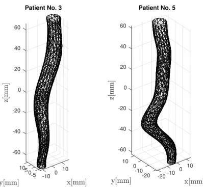
Generated meshes corresponding to the first phase are presented in Figure 1. The cross-sectional area is defined as the area of the section perpendicular to the center line of the fitted surface.

-60

105 10

-40

0 0-5 -10 -20

0

Patient No. 3

20 40 60

-60 10 -40

0 10

0 -20

-10 -10

-20 -20 0

Patient No. 5

20 40 60

Figure 1: 3D mesh models of a non-branching vessel segments in the thoracic aorta

3. Presentation and resolution of the inverse prob- lem

In this Section, we introduce the 1D blood flow model used in this study. We define the class of physically admissible solutions. We show that the volumetric flux can be calculated by solving a Riccati type ODE. We demonstrate that a physically admissible solution is not necessarily asymptotically stable. We will see that vessel wall motions do not provide enough information about the wall elasticity to recover the volumetric flux. We present a block-based optimization algorithm to resolve this problem.

3.1. Governing equations

To make our exposition self-contained and understandable for the largest possible audience, we present some laws of continuum mechanics: the conservation laws for mass and momentum. In addition, empirical constitutive laws are needed to relate certain unknown variables such as relations between stress and strain. Although there are one-dimensional models which also take into account fluid viscosity and wall viscoelasticity [15], we examine a simpler model using Euler’s equation for the non-viscose case. However, our approach can be generalized to more sophisticated

models involving damping effects. We assume that the vessel wall is thin and elastic.

Owing to the pressure gradient the artery wall deforms and the elastic restoring force of the wall makes it possible for waves to propagate and so it maintains a pulsating motion of the artery.

Now, we consider a non-branching cylindric vessel segment of length 𝐿. The section area𝑆(𝑡, 𝑧)and averaged flow velocity𝑢(𝑡, 𝑧)vary in time along the artery 𝑧 ∈ [0, 𝐿]. We define the volumetric flux as 𝑞 = 𝑢𝑆. Assuming that blood is homogeneous and incompressible, we obtain from the law for conversation of mass that

𝜕𝑡𝑆+𝜕𝑧𝑞= 0.

Additionally, the law for conservation of momentum has the following form

𝜕𝑡𝑢+𝑢𝜕𝑧𝑢=−𝜕𝑧𝑝

𝜌 , (3.1)

where 𝜌denotes the blood density and𝑝(𝑡, 𝑧)is the local blood pressure. We use the Hook’s law to relate stress and strain rates. Letℎbe the vessel wall thickness, assumed to be much smaller than the vessel radius, and Young’s modulus will be denoted by𝐸. The change in tube radius must be caused by the blood pressure.

The elastic strain due to the lengthening of the circumference is 𝑟(𝑡, 𝑧)−𝑟0(𝑧)

𝑟0(𝑧) ,

where𝑟0(𝑧)stands for the equilibrium radius. The change is elastic force must be balanced by the changing in pressure force2𝑟(𝑡, 𝑧)𝑝(𝑡, 𝑧), hence the desired relation between pressure and radius has the following form.

𝑝(𝑡, 𝑧) = (︂ 1

𝑟0(𝑧)− 1 𝑟(𝑡, 𝑧)

)︂

ℎ𝐸

For the right-hand side in (3.1), we obtain 𝑅𝛼(𝑡, 𝑧)^def.= −1

𝜌𝜕𝑧𝑝=𝛼

(︂ 𝑆₀^′(𝑧)

𝑆0(𝑧)^3/2 − 𝜕𝑧𝑆 𝑆(𝑡, 𝑧)^3/2

)︂

where 𝛼= 0.5ℎ𝐸𝜋^1/2𝜌⁻¹ is called wall compliance parameter and it is assumed to be constant during the cardiac cycle. By the conservation law for mass, the momentum transport equation can be expressed by means of the volumetric flux as follows:

𝜕𝑡𝑞+𝜕𝑧(︀

𝑞²/𝑆)︀

=𝑆(𝑡, 𝑧)𝑅𝛼(𝑡, 𝑧). (3.2)

3.2. Physically admissible solutions

Assuming that𝑆,𝑆0and𝛼are known, we are looking for special solutions of (3.2).

We will assume in the sequel that blood flows from𝑧= 0to𝑧=𝐿.

Definition 3.1. A solution𝑞of (3.2) is said to be physiologically admissible if it is periodic with period𝑇 and

𝑞min< 1 𝑇

∫︁𝑇 0

𝑞(𝑡, 𝑧) d𝑧 < 𝑞max

holds for 𝑧 ∈ [0, 𝐿], where 𝑞min and 𝑞max are the minimal and maximal average flow rate which may occur under physiological conditions.

Using the continuity law again, we can express the volumetric flux as 𝑞(𝑡, 𝑧) =𝑞(𝑡,0) + Φ(𝑡, 𝑧),

where 𝑄(𝑡) = 𝑞(𝑡,0) and Φ(𝑡, 𝑧) = −

∫︀𝑧 0

𝜕𝑡𝑆(𝑡, 𝑦) d𝑦. Note that the periodicity of 𝑆 implies that 𝑞 is physiologically admissible if and only if 𝑄 satisfies itself the conditions of admissibility.

After substituting the expression we have recently got for 𝑞 into (3.2) and integrating both sides from 0 to 𝐿, we get a Riccati type ODE with periodic coefficients

𝑄˙ =𝐴𝑄²+𝐵𝑄+𝐶, (3.3)

where dot denotes the time derivative and for the coefficients we have 𝐴(𝑡) =−1

𝐿

[︂ 1

𝑆(𝑡, 𝐿)− 1 𝑆(𝑡,0)

]︂

𝐵(𝑡) =−2 𝐿

Φ(𝑡, 𝐿) 𝑆(𝑡, 𝐿)

𝐶(𝑡) =−1 𝐿

⎡

⎣Φ²(𝑡, 𝐿) 𝑆(𝑡, 𝐿) +

∫︁𝐿 0

𝑆(𝑡, 𝑧) +𝑅𝛼(𝑡, 𝑧) d𝑧

⎤

⎦

It is a well known fact that the general solution of a scalar Riccati equation can be obtained by quadrature whenever at least one particular solution 𝑄0 is known.

After substituting 𝑄=𝑄0−1/𝑊 into the original equation, we get a linear ODE for𝑊:

𝑊˙ =−(2𝑄0𝐴+𝐵)𝑊 +𝐴 which general solution can be written as

𝑊(𝑡) =𝐾𝑊1(𝑡) +𝑊2(𝑡),

where 𝐾 is an arbitrary constant, 𝑊1(0) = 1 and 𝑊2(0) = 0. Periodicity of 𝑄 requires that 𝑄(0) = 𝑄(𝑇) which holds if and only if 𝐾 solves the quadratic equation:

𝑄0(𝑇)𝐾²+ (︂

𝑄0(𝑇)𝑊2(𝑇)

𝑊1(𝑇)−𝑊1(𝑇)−1 𝑊1(𝑇)

)︂

𝐾−𝑊2(𝑇)

𝑊1(𝑇) = 0 (3.4)

where we assumed that 𝑄0(0) = 0. We can conclude that the original Riccati equation has 0, 1 or 2 periodic solutions depending on the discriminant of equation (3.4). However, we need to know 𝑊1(𝑇), 𝑊2(𝑇) and𝑄0(𝑇)in order to calculate the discriminant and that can be done just for a given case.

Leon Kotin demonstrated the existence and uniqueness of a positive and of a negative periodic solution of a periodic Riccati equation in which the coefficients satisfy certain general condition. Moreover, any solution which is everywhere con- tinuous lies between these two solutions, and every solution is asymptotic to one of these as the independent variable increases or decreases [11]. More precisely, the following is true.

Theorem 3.2. If coefficients in(3.3)are continuous everywhere,𝐴is continuously differentiable and𝐴𝐶 <0holds, then equation (3.3)has a unique positive solution 𝑄+ and a unique negative solution𝑄₋ which are periodic with period 𝑇 and any solution behaves asymptotically like 𝑄+ or𝑄₋ as 𝑡→ ∞.

It is clear that if conditions of Kotin’s theorem are satisfied, then𝑄+ can be the unique physically admissible solution. However, the average volumetric flux calculated from𝑄+ may not fall into the acceptance interval. Moreover, nothing guarantees that𝑄+is asymptotically stable. For example, consider the case when 𝐶 < 0 and 𝑄 is an arbitrary perturbation of 𝑄+. From the uniqueness of the positive solution, we can conclude that there exists 𝑡0 ∈Rwhere 𝑄vanishes and 𝑄can have only one root, since at𝑄= 0the right-hand side of (3.3) is equal to𝐶 which is negative. As a consequence, we get that the physically admissible solution is not necessarily asymptotically stable.

3.3. Calculation of model parameters

For any fixed𝛼, we can calculate𝑊1,𝑊2and𝑄0numerically thus for the periodic solutions of (3.3)

𝑄1,2(𝑡) =𝑄0(𝑡)− 1

𝐾1,2𝑊1(𝑡) +𝑊2(𝑡)

yields, 𝐾1 where and𝐾2 are solutions of (3.4). However, we do not have a priori information about the wall compliance parameter hence the problem is undeter- mined.

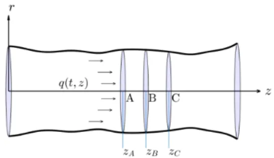
In order to reconstruct the volumetric flux from changes of the section area, we consider two adjacent vessel segment of length𝐿that are narrow enough to neglect the longitudinal changes in the artery wall compliance parameter. Now, we follow the notations of Figure 2, where 𝑧𝐶−𝑧𝐵 =𝑧𝐵−𝑧𝐴=𝐿and changes in between and are negligible.

If𝛼is fixed, then𝑞𝛼,1denotes the volumetric flow rate calculated from changes of the section area between 𝑧𝐴 and 𝑧𝐵 while 𝑞𝛼,2 stands for the volumetric flux obtained from the second vessel segment. For the true𝛼,𝑞𝛼,1(𝑡, 𝑧𝐵)and𝑞𝛼,2(𝑡, 𝑧𝐵) should be equal to each other for 𝑡 ∈ [0, 𝑇]. To measure the goodness of 𝛼, we

Figure 2: Blood flow in an arterial segment introduce the so-called internal consistency functional

𝐼𝛼=

∫︁𝑇 0

(𝑞𝛼,1(𝑡, 𝑧𝐵)−𝑞𝛼,2(𝑡, 𝑧𝐵))²d𝑡

that penalizes the difference between volumetric flow rates at 𝑧𝐵 obtained for the first and second vessel segment. We also introduce the notation

𝑉𝛼= 1 2𝑇

∫︁𝑇 0

𝑞𝛼,1(𝑡, 𝑧𝐵) +𝑞𝛼,2(𝑡, 𝑧𝐵) d𝑡

for the average volumetric flux at 𝑧𝐵. Therefore, we can formulate the original problem as a constrained minimization of𝐼𝛼.

min𝛼 𝐼𝛼

subject to 𝑞min< 𝑉𝛼< 𝑞max,

where the prescribed constraint ensures the physical admissibility of the solution.

The domain of 𝐼𝛼 consists of positive 𝛼 values for which Riccati equations related to the first and second vessel segment admits periodic solutions i.e. the discriminant of the corresponding quadratic equation is positive. Obviously, 𝑉𝛼

depends smoothly on𝛼hence the feasibility set of the optimization problem is an open set in (0,∞) which is a collection of open intervals. At this point, we do not have any further information about the structure of this set. We just assume during the simulations that it is connected i.e. it is an open interval. We will see in the next section that this assumption is justified by simulation results. So, we first solve non-linear scalar equations

𝑉𝛼=𝑞min, 𝑞max

for𝛼and get 𝛼min and𝛼max. After this, we calculate 𝛼_opt = arg min

𝛼∈(𝛼min,𝛼max)

𝐼𝛼. At least, the volumetric flux for the whole arterial segment can be obtained as

𝑞(𝑡, 𝑧) = 1 2

(︀𝑞𝛼_opt,1(𝑡, 𝑧) +𝑞𝛼_opt,2(𝑡, 𝑧))︀

.

In our MATLAB implementation, we used the ode45 function to solve ini- tial value problems, fzero function to solve non-linear equations for values cor- responding to the minimal and maximal flow rate. At least, we applied the fminbnd function to find the global minimum of on. More information about these MATLAB solvers is available in the online MATLAB documentation: https:

//www.mathworks.com/help/matlab/.

4. Results

Numerical simulations were performed on a10cm long non-branching segment in the descending aorta, where the𝑧= 0level is located1cm below the heart. In order to minimize the disturbing effect of moving organs, we chose the last2×1cm region which means that we set𝑧𝐴= 8cm, 𝑧𝐵= 9cm and𝑧𝐶 = 10cm. According to the medical literature, cardiac output lies between 4dm³/min and 6dm³/min hence we set the maximal and minimal average flow rate to 66.7cm³/s and 100cm³/s, respectively. We defined the equilibrium cross-sectional area as

𝑆0(𝑧) = min

𝑡∈[0,𝑇]𝑆(𝑡, 𝑧).

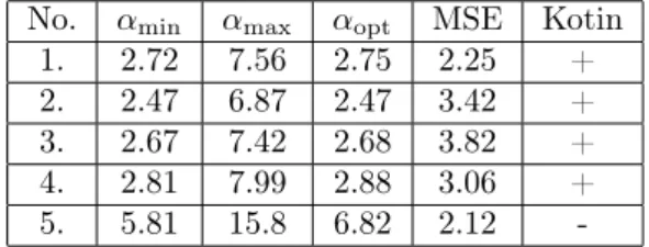
We summarize the simulation results in Table 2, where mean squared error is defined as MSE=(︀

𝐼𝛼_opt/𝑇)︀1/2

and it characterizes the goodness of the optimum.

No. 𝛼min 𝛼max 𝛼opt MSE Kotin

1. 2.72 7.56 2.75 2.25 +

2. 2.47 6.87 2.47 3.42 +

3. 2.67 7.42 2.68 3.82 +

4. 2.81 7.99 2.88 3.06 +

5. 5.81 15.8 6.82 2.12 -

Table 2: Wall compliance parameter values (10³cm³/s²) , mean squared error(cm³/s)and conditions of Kotin’s theorem – satisfied

(+) or not (-)

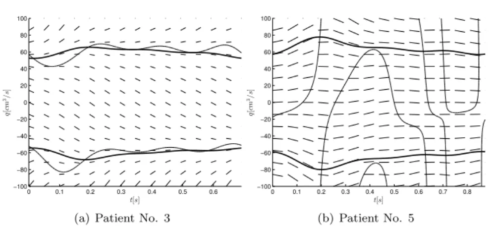
We can see that conditions of Kotin’s theorem are satisfied in all cases except for the oldest participant. We present phase portraits of the Riccati equation corresponding to the youngest and oldest participants (Figure 3A and 3B). Phase portrait presented in Figure 3a exhibits the typical behavior. We got similar results for patient No. 1, 2 and 4. In this case, we can realize that the only positive and physiologically admissible solution is unstable which is contrary to intuition. It is not clear at this point if exists any relationship between the qualitative behavior of solutions and arterial wall rigidity. Such connection would be helpful in order to gain information about the condition of the circulatory system and detect vascular diseases.

We calculated the volumetric flux at three different longitudinal position along- side the artery segment: 𝑧1 = 1cm, 𝑧2 = 5cm and𝑧3 = 9cm. Simulation results

0 0.1 0.2 0.3 0.4 0.5 0.6

−100

−80

−60

−40

−20 0 20 40 60 80 100

t[s]

q[cm3/s]

(a) Patient No. 3

0 0.1 0.2 0.3 0.4 0.5 0.6 0.7 0.8

−100

−80

−60

−40

−20 0 20 40 60 80 100

t[s]

q[cm3/s]

(b) Patient No. 5

Figure 3: Phase portrait of the typical and non-typical behavior

for patient No. 3 are presented in Figure 4. As we are getting further from the beating heart and approaching the aortic bifurcation, initial peak in the volumet- ric flux slowly disappears and reflections from the arteria iliaca became even more dominant.

0 20 40 60 80 100

52 54 56 58 60 62 64 66 68 70

Figure 4: Volumetric flux(︀cm³/s)︀vs. time (% of the cardiac cycle):

blue–𝑧1= 1cm, green–𝑧2= 5cm, red–𝑧3= 9cm

The remaining part of this section is devoted to the analysis of the velocity profile inside the aorta by means of Reynolds and Womersley numbers. For the sake of completeness, we give here the definitions of these dimensionless numbers.

The Reynolds number is a dimensionless number in fluid mechanics that is defined

as the ratio of inertia forces to viscous forces, expressed in tubular flows as Re= 2𝑣𝑟𝜌

𝜂 ,

where 𝑣 is the flow velocity, 𝑟 is the vessel radius,𝜌is the blood density and𝜂 is the dynamical viscosity of blood. The Womersley number in biofluid mechanics relates the transient inertial forces to viscous effects. It is defined by

Wh= 2𝑟

√︂𝜔𝜌 𝜂 ,

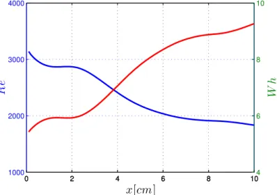
where𝜔 is the angular frequency of the oscillations. In accordance with the litera- ture [7, 8], in our calculations blood density was set to1.06g/cm³and the kinematic viscosity of blood to 3.5×10⁻³ Pas. Estimations for Reynolds and Womersley numbers along the artery segment are illustrated in common coordinate system in Figure 5.

0 2 4 6 8 10

1000 2000 3000 4000

x[cm]

Re

0 2 4 6 8 10

4 6 8 10

Wh

Figure 5: Time average of Reynolds and Womerseley numbers

The Womersley number is a dynamic similarity measure of oscillatory flows relating inertia and viscous forces. In rigid pipes for laminar incompressible flows small values (approx. Wh < 1) allow the development of the parabolic velocity profile of the steady state solution and the flow is almost in phase with the pressure gradient, while large values (approx. Wh > 10) indicate a flat velocity profile with a good approximation and the flow follows the pressure gradient by about 90 degrees in phase. In the presented examples – as seen in Figure 5 – the values lie in between, yielding a complex time-dependent velocity profile. The Reynolds number is another dynamic similarity measure relating inertia and viscous forces.

In rigid pipes small values (approx. Re<2100) indicate laminar flow, while large

values (approx. Re>4000) correspond to turbulent flow. In the transition zone, where also our example is situated, the behavior strongly depends on the existing disturbances in the flow.

5. Conclusions

The inverse problem for volumetric flow rate reconstruction in large arteries has been successfully solved. We demonstrated that in the majority of cases periodic so- lutions are unstable even though the changes of the cross-sectional area is supposed to be periodic in time. Our approach makes possible to calculate the aortic flow on a routine ECG-gated CT angiography dataset. This is of huge clinical poten- tial, as the knowledge of haemodynamic parameters could significantly improve the diagnostic performance of CT imaging in several cardiovascular pathologies, such as aortic coarctation or dissection. However, further verifications and comparative studies are needed to validate our method in a clinical cohort.

References

[1] J. Alastruey,K. H. Parker,S. J. Sherwin:Arterial pulse wave haemodynamics, in:

11th International Conference on Pressure Surges, Virtual PiE Led t/a BHR Group, 2012, pp. 401–443,isbn: 9781855981331.

[2] J. Alastruey,N. Xiao,H. Fok,T. Schaeffter,C. A. Figueroa:On the impact of mod- elling assumptions in multi-scale, subject-specific models of aortic haemodynamics, Journal of The Royal Society Interface 13.119 (2016),issn: 1742-5689,doi:10.1098/rsif.2016.0073, eprint: http://rsif.royalsocietypublishing.org/content/13/119/20160073.full.pdf, url:http://rsif.royalsocietypublishing.org/content/13/119/20160073.

[3] C. R. Becker,B. M. Ohnesorge,U. J. Schoepf,M. F. Reiser:Current development of cardiac imaging with multidetector-row CT, European Journal of Radiology 36.2 (2000), pp. 97–103,doi:10.1016/S0720-048X(00)00272-2.

[4] L. Dumas:Inverse problems for blood flow simulation, in: Proceedings of EngOpt2008 – International Conference on Engineering Optimization, 2008.

[5] J. P. Earls,E. L. Berman,B. A. Urban, et al.:Prospectively Gated Transverse Coro- nary CT Angiography versus Retrospectively Gated Helical Technique: Improved Image Qual- ity and Reduced Radiation Dose, Radiology 246.3 (2008), pp. 742–753,doi:10.1148/radiol.

2463070989.

[6] L. Euler:Principia pro motu sanguinis per arterias determinando, Opera posthuma math- ematica et physica anno 1844 detecta 2 (1775), pp. 814–823.

[7] H. Hinghofer-Szalkay,J. E. Greenleaf:Continuous monitoring of blood volume chan- ges in humans, Journal of Applied Physiology 63.3 (1987), pp. 1003–1007,doi:10.1152/

jappl.1987.63.3.1003.

[8] J. M. Jung,D. H. Lee,K. T. Kim, et al.:Reference intervals for whole blood viscos- ity using the analytical performance-evaluated scanning capillary tube viscometer, Clinical Biochemistry 47.6 (2014), pp. 489–493,doi:10.1016/j.clinbiochem.2014.01.021.

[9] M. Kass,A. P. Witkin,D. Terzopoulos:Snakes: Active contour models, International Journal of Computer Vision 1.4 (1988), pp. 321–331,doi:10.1007/BF00133570.

[10] D. J. Korteweg:Ueber die Fortpflanzungsgeschwindigkeit des Schalles in elastischen Röh- ren, Annalen der Physik 241.12 (1878), pp. 525–542,doi:10.1002/andp.18782411206.

[11] L. Kotin:On Positive and Periodic Solutions of Riccati Equations, SIAM Journal of Applied Mathematics 16.6 (1968), pp. 1227–1231,doi:10.1137/0116103.

[12] H. Lamb: On the velocity of sound in a tube, as affected by the elasticity of the walls, Manchester Memoirs 42 (1898), pp. 1–16.

[13] R. Nagy,Cs. Csobay-Novák,A. Lovas,S. Péter,I. Bojtár:Non-invasive in vivo time- dependent strain measurement method in human abdominal aortic aneurysms: Towards a novel approach to rupture risk estimation, Journal of biomechanics 48.10 (2015), pp. 1876–

1886,doi:10.1016/j.jbiomech.2015.04.030.

[14] M. Sonka,V. Hlaváč,R. Boyle:Image Processing, Analysis, and Machine Vision, ISBN- 10: 1133593607, Cengage Learning, 2008,doi:10.1007/978-1-4899-3216-7.

[15] X. Wang,S. Nishi,M. Matsukawa, et al.:Fluid friction and wall viscosity of the 1D blood flow model, Journal of biomechanics 49 (4 2016), pp. 565–571, doi:10.1016/j.jbiomech.

2016.01.010.