Distance-based accessibility indices
by László Csató
C O R VI N U S E C O N O M IC S W O R K IN G P A PE R S
CEWP 12 /201 5
Distance-based accessibility indices *
L´ aszl´ o Csat´ o
†Department of Operations Research and Actuarial Sciences Corvinus University of Budapest
MTA-BCE ”Lend¨ulet” Strategic Interactions Research Group Budapest, Hungary
June 30, 2015
Abstract
The paper attempts to develop a suitable accessibility index for networks where each link has a value such that a smaller number is preferred like distance, cost, or travel time. A measure called distance sum is characterized by three independent properties: anonymity, an appropriately chosen independence axiom, and dominance preservation, which requires that a node not far to any other is at least as accessible.
We argue for the need of eliminating the independence property in certain applications. Therefore generalized distance sum, a family of accessibility indices, will be suggested. It is linear, considers the accessibility of vertices besides their distances and depends on a parameter in order to control its deviation from distance sum. Generalized distance sum is anonymous and satisfies dominance preservation if its parameter meets a sufficient condition. Two detailed examples demonstrate its ability to reflect the vulnerability of accessibility to link disruptions.
JEL classification number: D85, Z13
Keywords: Networks, Geography, Accessibility, Distance sum, Axiomatic approach
1 Introduction
Section1aims to confirm the importance of accessibility indices. Some applications of them are presented in Subsection 1.1together with a detailed literature review in Subsection1.2.
Finally, Subsection 1.3 gives an outline of our approach and main results.
1.1 Motivation
A key and basic concept in network analysis that researchers want to capture is centrality.
The well-known classification ofFreeman (1979) distinguishes three conceptions, measured
* We are grateful to Dezs˝o Bednay for useful advices.
The research was supported by OTKA grant K 111797 and MTA-SYLFF (The Ryoichi Sasakawa Young Leaders Fellowship Fund) grant ’Mathematical analysis of centrality measures’, awarded to the author in 2015.
† e-mail: laszlo.csato@uni-corvinus.hu
by degree, closeness, and betweenness, respectively. However, there is a frequent need for other centrality models. One of them, mainly used in theoretical geography for analysing social activities and regional economies, can be called accessibility. Accessibility index provides a numerical answer to questions such as ’How accessible is a node from other nodes in a network?’ or ’What is its relative geographical importance?’.
Accessibility measures have a number of interesting ways of utilization:
1. Knowledge of which nodes have the highest accessibility could be of interest in itself (e.g. by revealing their strategic importance);
2. The accessibility of vertices could be statistically correlated to other economic, sociological or political variables;
3. Accessibility of the same nodes (e.g. urban centers) in different (e.g. transportation, infrastructure) networks could be compared;
4. Proposed changes in a network could be evaluated in terms of their effect on the accessibility of vertices;
5. Networks (e.g. empires) could be compared by their propensity to disintegrate. For example, it may be difficult to manage from a unique centre if the most accessible nodes are far from each other.
Practical application of accessibility involve, among others, an analysis of the medieval river trade network of Russia (Pitts, 1965, 1979), of the medieval Serbian oecumene (Carter, 1969), of the interstate highway network for cities in the southeastern United States (Garrison, 1960; Ma´ckiewicz and Ratajczak, 1996), of the inter-island voyaging network of the Marshall islands (Hage and Harary, 1995), or of the global maritime container transportation network (Wang and Cullinane, 2008). Accessibility indices can be used in operations research, too, where a typical problem is that of choosing a site for a facility on the basis of a specific criterion (Slater, 1981).
1.2 Some methods for measuring accessibility
The adjacency matrix 𝐶 of the network graph is given by𝑐𝑖𝑗 = 1 if and only if nodes 𝑖 and 𝑗 are connected and 𝑐𝑖𝑗 = 0 otherwise.
One of the first accessibility indices, sometimes calledconnection array, was introduced by Garrison(1960). It is based on powering of matrix 𝐶 such that
𝑇 =𝐶+𝐶2 +𝐶3+· · ·+𝐶𝑚 =
𝑚
∑︁
𝑖=1
𝐶𝑖.
The accessibility of a node comes from summing the corresponding column of matrix𝑇, i.e. the total number of at most 𝑚-long paths to other nodes. It was used by Pitts (1965) and Carter (1969) despite two significant shortcomings:
∙ The increase of 𝑚 distorts reality as some redundant paths (i.e. longer than the shortest path in a topological sense) are included in the calculation of accessibility.
∙ It is not obvious what is the appropriate value of 𝑚. The usual choice is the diameter, the maximum number of edges in the shortest path between the furthest pair of nodes, which provides that 𝑇 has only positive elements (if 𝑚 ≥2).
The first problem may be addressed by introducing a multiplier for𝐶𝑖 showing exponential decay in the calculation of matrix 𝑇, as suggested by Garrison (1960) following Katz (1953). However, it is still not able to completely overcome the inherent failures of the
method (Ma´ckiewicz and Ratajczak,1996).
In order to improve the comparability of results achieved for various𝑚, Stutz (1973) proposed a formula to determine the relative accessibility of nodes.
Naturally, one can focus only on the shortest paths between the nodes. Then a plausible measure is the total length of them to all other nodes (Shimbel, 1951,1953;Harary, 1959;
Pitts,1965;Carter, 1969), which is called shortest-path array.
Betweenness measures how many shortest paths pass through the given node (Shimbel, 1953;Freeman, 1977). It was also applied as an accessibility index (Pitts, 1979).
Eccentricity concentrates on the maximum distance to all other nodes. Sometimes it is the suitable concept for predicting the politically and symbolically important nodes in a network (Hage and Harary, 1995).
A whole branch of literature, initiated by (Gould, 1967), propagates the use of eigen- vectors for measuring accessibility (Carter, 1969;Tinkler, 1972; Straffin, 1980; Ma´ckiewicz and Ratajczak, 1996; Wang and Cullinane, 2008). It is based on the Perron-Frobenius theorem (Perron, 1907; Frobenius, 1908, 1909, 1912) for nonnegative square matrices:
matrix 𝐶 has a unique (up to constant multiples) positive eigenvector corresponding to the principal eigenvalue. It have been proposed that the non-principal eigenvectors might also have geographical meaning, however, its use remains controversial (Carter,1969;Hay, 1975;Tinkler, 1975; Straffin,1980).
Finally, Amer et al. (2012) construct accessibility indices to the nodes of directed graphs using methods of game theory.
1.3 Aims and tools
The focus on the adjacency matrix has no sense in some applications, where the network graph is closely complete (Wang and Cullinane,2008). However, asTaaffe and Gauthier (1973) claim, it is not necessary to restrict the concept to a purely topological one. Value of linkages may be given as a distance between the nodes in actual mileage as well as the cost of movement or the time required to travel between them. Actually, it was implemented by Carter(1969) and Pitts (1979) using the distance as a value.
We will call the edge valuesdistance throughout the paper. It may be any measure satisfying triangle inequality such that a smaller value is better. It can be assumed without loss of generality that the network is complete, i.e. a value is available for each link. While the extension of shortest-path array to this domain, said to be the distance sum, is obvious, the applicability of other measures – presented in Subsection 1.2 – is ambiguous, despite the use of the principal eigenvector by Wang and Cullinane (2008).
The paper aims to analyse accessibility indices in these networks. For this purpose the axiomatic approach, a standard path in game and social choice theory will be applied.
Distance sum will be characterized, that is, a set of properties will be given such that it is the only accessibility index satisfying them, but eliminating any axiom allows for other measures. According to our knowledge, no axiomatizations of accessibility indices exist.
However, some results are provided for other centrality measures (Monsuur and Storcken, 2004; Garg, 2009;Kitti, 2012; Dequiedt and Zenou, 2014).
The characterization of distance sum, one of the main results, contains three axioms:
anonymity, an appropriately chosen independence axiom (independence of distance dis- tribution), and dominance preservation, which requires that a node not far to any other is at least as accessible. Furthermore, it will be presented through an example that independence of distance distribution is a property one would rather not have in certain cases. Therefore a parametric family of accessibility indices will be proposed.
It will be called generalized distance sum as it redistributes the pool of aggregated distances (i.e. the sum of distances over the network) by considering distance distribution:
in the case of two nodes with the same distance sum, it is deemed better to be close to more accessible nodes (and therefore, to be far to less accessible ones) than vice versa. It also takes into account – similarly to connection array – longer paths than the shortest, their impact is governed by the parameter. The main argument for their inclusion is that shortest paths may be vulnerable to disruptions, when the value of alternative routes becomes relevant. The limit of generalized distance sum is the distance sum.
Generalized distance sum satisfies anonymity and violates independence of distance distribution. The other main result provides a sufficient condition for this measure – by limiting the value of its parameter – to meet dominance preservation, the third axiom in the characterization of distance sum. However, it will not be axiomatized.
While it is not debated that characterizations are a correct way to distinguish between accessibility indices, we think they have limited significance for applications: if one should determine the accessibilities in a given network, he/she is not much interested in the properties of the measure on other networks. Characterizations could reveal some aspects of the choice but the consequences of the axioms on the actual network remain obscure.
The axiomatic point of view is not exclusive. Borgatti and Everett(2006) criticize this way, taken by Sabidussi (1966), because it does not ’actually attempt to explain what centrality is’. Thus generalized distance sum will be scrutinized through some examples, showing that it is able to reflect the structure of the network.
The paper is structured as follows. Section2 describes the characterization of distance sum. Subsection2.1defines the model and the accessibility index. Subsection2.2is devoted to introduce the axioms and to prove the theorem as well as to discuss the independence of properties and an extension of the result. Section 3 presents a new parametric measure of accessibility by challenging an axiom of the previous characterization. Generalized distance sum is motivated and introduced in Subsection 3.1. We also deal with some of its properties and return to address triangle inequality, a potential constraint of the model. Subsection 3.2gives a sufficient condition for generalized distance sum to satisfy another property used in the axiomatization. It is shown that an excessive value of the parameter may lead to counter-intuitive accessibility rankings. Two examples are discussed in Subsection 3.3 to reveal some interesting feature of the suggested measure. Sections 2 and 3contain somewhat independent results, the axiomatization of distance sum is wholly autonomous, and generalized distance sum may be submitted and discussed without the characterization, too. Finally, Section 4 summarizes our findings and outlines some directions for future research.
2 A characterization of distance sum
In this section, some natural conditions will be conceived for accessibility indices, similarly to centrality measures (Sabidussi,1966;Chien et al.,2004;Landherr et al.,2010;Boldi and Vigna, 2014). Distance sum, an obvious solution for our problem, will be characterized, that is, a set of properties will be given such that it is the only accessibility index satisfying them, while eliminating any axiom allows for other measures.
2.1 The model
Definition 1. Transportation network: Transportation network is a pair (𝑁, 𝐷) such that
∙ 𝑁 ={1,2, . . . , 𝑛} is a finite set of nodes;
∙ 𝐷∈R𝑛×𝑛+ is a symmetric distance matrix satisfying triangle inequality, namely, 𝑑𝑖𝑗 ≤∑︀𝑚−1ℓ=0 𝑑𝑘ℓ𝑘ℓ+1 where (𝑖=𝑘0, 𝑘1, . . . , 𝑘𝑚 =𝑗) is a path between the nodes 𝑖 and 𝑗. 𝑑𝑖𝑖= 0 for all𝑖= 1,2, . . . , 𝑛.
𝐷 can be the adjacency matrix of a complete, weighted, undirected graph (without loops and multiple edges) with the set of nodes 𝑁.1
Notation 1. 𝒩𝑛 is the class of all transportation networks (𝑁, 𝐷) with |𝑁|=𝑛.
Definition 2. Accessibility index: Let (𝑁, 𝐷) ∈ 𝒩𝑛 be a transportation network. Ac- cessibility index 𝑓 is a function that assigns an 𝑛-dimensional vector of real numbers to (𝑁, 𝐷) with 𝑓𝑖(𝑁, 𝐷) showing the accessibility of node 𝑖.
Notation 2. 𝑓 :𝒩𝑛→R𝑛 is an accessibility index.
Node𝑖is said to be at least as accessible as node𝑗 in the transportation network (𝑁, 𝐷) if and only if 𝑓𝑖(𝑁, 𝐷)≤𝑓𝑗(𝑁, 𝐷), so a smaller value of accessibility is more favourable.
Definition 3. Order equivalence: Let𝑓, 𝑔 :𝒩𝑛→R𝑛 be two accessibility indices. They are called order equivalent if and only if 𝑓𝑖(𝑁, 𝐷)≤𝑓𝑗(𝑁, 𝐷)⇔𝑓𝑖(𝑁, 𝐷)≤𝑓𝑗(𝑁, 𝐷) for any transportation network (𝑁, 𝐷)∈ 𝒩𝑛. .
Notation 3. 𝑓 ≈𝑔 means that accessibility measures𝑓, 𝑔 :𝒩𝑛→R𝑛 are order equivalent.
Since we focus on accessibility rankings, order equivalent accessibility indices are not distinguished. For example, an accessibility index is invariant under multiplication by positive scalars.
Throughout the paper, vectors are denoted by bold fonts and assumed to be column vectors. Let e ∈ R𝑛 be the column vector such that 𝑒𝑖 = 1 for all 𝑖 = 1,2, . . . , 𝑛 and 𝐼 ∈R𝑛×𝑛 be the matrix with 𝐼𝑖𝑗 = 1 for all 𝑖, 𝑗 = 1,2, . . . , 𝑛.
The first, almost trivial idea to measure accessibility can be the sum of distances to all other nodes. In fact, it is extensively used in the literature (Shimbel, 1951, 1953; Harary, 1959;Pitts,1965;Carter, 1969).
Definition 4. Distance sum: dΣ :𝒩𝑛→R𝑛 such that 𝑑Σ𝑖 =∑︀𝑗∈𝑁𝑑𝑖𝑗 for all 𝑖∈𝑁.
1 Assumption of completeness is not restrictive in the case of connected graphs since the distance of any pair of nodes can be measured by the shortest path between them.
2.2 Axioms and characterization
The first condition is independence of the labelling of the nodes.
Definition 5. Anonymity (𝐴𝑁 𝑂): Let (𝑁, 𝐷),(𝜎𝑁, 𝜎𝐷) ∈ 𝒩 be two transportation networks such that (𝜎𝑁, 𝜎𝐷) is given by a permutation of nodes 𝜎 :𝑁 →𝑁 from (𝑁, 𝐷).
Accessibility index 𝑓 :𝒩𝑛 → R𝑛 is called anonymous if 𝑓𝑖(𝑁, 𝐷) =𝑓𝜎𝑖(𝜎𝑁, 𝜎𝐷) for all 𝑖∈𝑁.
Property𝐴𝑁 𝑂implies that two symmetric nodes are equally accessible. It also ensures that all nodes have the same accessibility in a transportation network with the same distance between any pair of nodes.
Lemma 1. Distance sum satisfies 𝐴𝑁 𝑂.
While distance sum is usually a good baseline to approximate accessibility, it does not consider the distribution of distances.
Definition 6. Independence of distance distribution (𝐼𝐷𝐷): Let (𝑁, 𝐷) ∈ 𝒩𝑛 be a transportation network and 𝑖, 𝑗, 𝑘, ℓ∈𝑁 be four distinct nodes. Let𝑓 :𝒩𝑛 →R𝑛 be an accessibility index such that 𝑓𝑖(𝑁, 𝐷)≤𝑓𝑗(𝑁, 𝐷) and (𝑁, 𝐷′)∈ 𝒩𝑛 be a transportation network identical to (𝑁, 𝐷) except for 𝑑′𝑖𝑘 ̸=𝑑𝑖𝑘 and 𝑑′𝑖ℓ̸=𝑑𝑖ℓ but 𝑑′𝑖𝑘+𝑑′𝑖ℓ=𝑑𝑖𝑘+𝑑𝑖ℓ. 𝑓 is calledindependent of distance distribution if 𝑓𝑖(𝑁, 𝐷′)≤𝑓𝑗(𝑁, 𝐷′).
Property 𝐼𝐷𝐷 implies that the accessibility ranking does not change if the distance sum of each node remains the same.
Lemma 2. Distance sum satisfies 𝐼𝐷𝐷.
Definition 7. Dominance: Let (𝑁, 𝐷)∈ 𝒩𝑛 be a transportation network and 𝑖, 𝑗 ∈ 𝑁 be two distinct nodes such that 𝑑𝑖𝑘 ≤𝑑𝑗𝑘 for all𝑘 ∈𝑁∖ {𝑖, 𝑗} with a strict inequality (<) for at least one 𝑘.
Then it is said that node𝑖 dominates node 𝑗.
A natural requirement for accessibility indices can be that the accessibility of ’obviously’
more external nodes is worse.
Definition 8. Dominance preservation (𝐷𝑃): Let (𝑁, 𝐷) ∈ 𝒩𝑛 be a transportation network and 𝑖, 𝑗 ∈𝑁 be two distinct nodes such that node 𝑖 dominates node𝑗.
Accessibility index 𝑓 :𝒩𝑛 →R𝑛 preserves dominance if 𝑓𝑖(𝑁, 𝐷)< 𝑓𝑗(𝑁, 𝐷).
Property 𝐷𝑃 demands that if node𝑗 is at least as far from all nodes as node 𝑖, then it has a larger accessibility value provided that they could not be labelled arbitrarily. A similar axiom called self-consistency has been suggested by (Chebotarev and Shamis,1997) for preference aggregating methods.
Lemma 3. Distance sum satisfies 𝐷𝑃.
Requirements𝐴𝑁 𝑂, 𝐼𝐷𝐷 and 𝐷𝑃 still give a characterization of distance sum.
Theorem 1. If an accessibility index𝑓 :𝒩𝑛 →R𝑛 is anonymous, independent of distance distribution and preserves dominance, then 𝑓 is the distance sum.
Proof. Consider a transportation network (𝑁, 𝐷)∈ 𝒩𝑛and three nodes 𝑖, 𝑗, 𝑘∈𝑁. It can be assumed that∑︀𝑚∈𝑁𝑑𝑖𝑚≤∑︀𝑚∈𝑁𝑑𝑗𝑚. Define the transportation network (𝑁, 𝐷′)∈ 𝒩𝑛 such that𝑑′𝑖𝑚= 𝑑𝑖𝑚for all𝑚 ∈𝑁,𝑑′𝑗𝑘 =𝑑′𝑖𝑘+(∑︀𝑚∈𝑁 𝑑𝑗𝑚−∑︀𝑚∈𝑁𝑑𝑖𝑚)≤𝑑′𝑖𝑘 and𝑑′𝑗ℓ =𝑑′𝑖ℓ for all ℓ∈𝑁 ∖ {𝑖, 𝑗, 𝑘}. Two cases can be distinguished:
∙ ∑︀𝑚∈𝑁𝑑𝑖𝑚<∑︀𝑚∈𝑁 𝑑𝑗𝑚
Then 𝑑′𝑖𝑘 < 𝑑′𝑗𝑘, so 𝑓𝑖(𝑁, 𝐷′) < 𝑓𝑗(𝑁, 𝐷′) due to 𝐷𝑃 and 𝑓𝑖(𝑁, 𝐷)< 𝑓𝑗(𝑁, 𝐷) because of 𝐼𝐷𝐷 as ∑︀𝑚∈𝑁 𝑑′𝑖𝑚=∑︀𝑚∈𝑁𝑑𝑖𝑚 and ∑︀𝑚∈𝑁𝑑′𝑗𝑚 =∑︀𝑚∈𝑁𝑑𝑗𝑚.
∙ ∑︀𝑚∈𝑁𝑑𝑖𝑚=∑︀𝑚∈𝑁 𝑑𝑗𝑚
Then 𝑑′𝑖𝑘 =𝑑′𝑗𝑘, so 𝑓𝑖(𝑁, 𝐷′) =𝑓𝑗(𝑁, 𝐷′) due to 𝐴𝑁 𝑂 and 𝑓𝑖(𝑁, 𝐷) =𝑓𝑗(𝑁, 𝐷) because of 𝐼𝐷𝐷 as ∑︀𝑚∈𝑁 𝑑′𝑖𝑚=∑︀𝑚∈𝑁𝑑𝑖𝑚 and ∑︀𝑚∈𝑁𝑑′𝑗𝑚 =∑︀𝑚∈𝑁𝑑𝑗𝑚.
It implies that𝑓 ≈dΣ.
Remark 1. The proof of Theorem1 requires at least three nodes. However, 𝐼𝐷𝐷 has a meaning only for four nodes. It can be seen that𝐴𝑁 𝑂 and𝐷𝑃 are enough to characterize distance sum if 𝑛 = 3 since 𝑑𝑖𝑘 < 𝑑𝑗𝑘 ⇒ 𝑓𝑖(𝑁, 𝐷) < 𝑓𝑗(𝑁, 𝐷) because of dominance preservation and 𝑑𝑖𝑘 = 𝑑𝑗𝑘 ⇒ 𝑓𝑖(𝑁, 𝐷) = 𝑓𝑗(𝑁, 𝐷) due to anonymity. Note that 𝑑𝑖𝑗 ≤ 𝑑𝑖𝑘 ⇔∑︀𝑚∈𝑁𝑑𝑖𝑚≤∑︀𝑚∈𝑁𝑑𝑗𝑚 by definition.
Now the independence of the axioms is addressed.
Proposition 1. Anonymity, independence of distance distribution and domination preser- vation are logically independent conditions.
Proof. As usual, an example will be given that satisfies all the axioms mentioned in Theorem 1except for the one under consideration. Consider the following three functions:
Definition 9. Distance sum without ties: dΣ< : 𝒩𝑛 → R𝑛 such that𝑑Σ<𝑖 = ∑︀𝑗∈𝑁𝑑𝑖𝑗 + (𝑖−1) min{∑︀ℓ∈𝑁(𝑑𝑗ℓ−𝑑𝑘ℓ) :𝑗, 𝑘 ∈𝑁}/𝑛 for all 𝑖∈𝑁.
Definition 10. Inverse distance sum: d−Σ :𝒩𝑛 → R𝑛 such that 𝑑−Σ𝑖 =−∑︀𝑗∈𝑁𝑑𝑖𝑗 for all 𝑖∈𝑁.
Definition 11. Distance product: dΠ :𝒩𝑛→R𝑛 such that𝑑Π𝑖 =∏︀𝑗̸=𝑖𝑑𝑖𝑗 for all 𝑖∈𝑁. Distance sum without ties satisfies𝐼𝐷𝐷 and 𝐷𝑃 but violates 𝐴𝑁 𝑂 as in the case of equal distance sums, the node with a lower index becomes more accessible.
Inverse distance sum satisfies𝐴𝑁 𝑂 and 𝐼𝐷𝐷 but violates 𝐷𝑃.
Distance product satisfies𝐴𝑁 𝑂 and 𝐷𝑃 but it is not equivalent to distance sum.
Figure 1: Transportation network of Example 1 1
2 3
4 3
6 3
1
3 5
Example 1. Consider the transportation network (𝑁, 𝐷)∈ 𝒩4 in Figure 1 where dΣ(𝑁, 𝐷) =[︁ 9 10 9 14 ]︁⊤ and dΠ(𝑁, 𝐷) = [︁ 27 18 15 90 ]︁⊤. Note that 𝑑Σ1(𝑁, 𝐷)< 𝑑Σ2(𝑁, 𝐷) and 𝑑Π1(𝑁, 𝐷)> 𝑑Π2(𝑁, 𝐷).
Remark 2. Theorem 1 and Proposition 1 reveal a possible way to characterize inverse distance sum by 𝐴𝑁 𝑂,𝐼𝐷𝐷 and ’inverse’ domination preservation (i.e. with an opposite implication compared to 𝐷𝑃).
On the other hand, distance product can be axiomatized by 𝐴𝑁 𝑂, a modification of𝐼𝐷𝐷 such that the product of distances – instead of their sum – remains unchanged, and 𝐷𝑃.
3 The suggested measure: generalized distance sum
From the three axioms of Theorem 1, independence of distance distribution seems to be the less plausible. Therefore it is worth to examine its substitution by other considerations.
In this section a new accessibility index will be introduced and analysed with respect to its properties, especially dominance preservation.
3.1 The new accessibility index
𝐼𝐷𝐷 could be eliminated by the use distance product, for instance. However, the major disadvantage of distance sum may be that indirect connections are not taken into account, captured by the following condition.
Definition 12. Independence of irrelevant distances (𝐼𝐼𝐷): Let (𝑁, 𝐷) ∈ 𝒩𝑛 be a transportation network and 𝑖, 𝑗, 𝑘, ℓ∈𝑁 be four distinct nodes. Let𝑓 :𝒩𝑛 →R𝑛 be an accessibility index such that 𝑓𝑖(𝑁, 𝐷)≤𝑓𝑗(𝑁, 𝐷) and (𝑁, 𝐷′)∈ 𝒩𝑛 be a transportation network identical to (𝑁, 𝐷) except for 𝑑′𝑘ℓ ̸=𝑑𝑘ℓ.
𝑓 is calledindependent of irrelevant distances if 𝑓𝑖(𝑁, 𝐷′)≤𝑓𝑗(𝑁, 𝐷′).
It means that the relative accessibility of two nodes is not affected by the distances between other nodes. Independence of irrelevant distances is an adaptation of the axiom independence of irrelevant matches defined for (general) tournaments (Rubinstein, 1980;
Gonz´alez-D´ıaz et al., 2014).
Lemma 4. Distance sum, distance sum without ties, inverse distance sum and distance product meet 𝐼𝐼𝐷.
Definition 13. Shortest path-based accessibility index: Let (𝑁, 𝐷) ∈ 𝒩𝑛 be any trans- portation network.
Accessibility index 𝑓 : 𝒩𝑛 → R𝑛 is called a shortest path-based accessibility index if it satisfies independence of irrelevant distances.
Remark 3. Distance sum, distance sum without ties, inverse distance sum and distance product are shortest path-based accessibility indices.
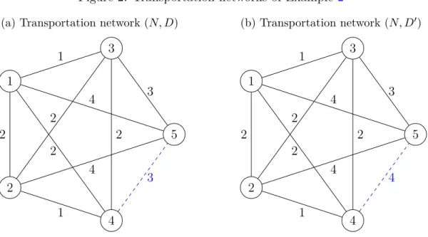
Figure 2: Transportation networks of Example2 (a) Transportation network (𝑁, 𝐷)
1
2
3
4
5 1
1 2 2
3
3 4
4
2 2
(b) Transportation network (𝑁, 𝐷′)
1
2
3
4
5 1
1 2 2
3
4 4
4
2 2
A shortest path-based accessibility index considers only the local structure of the network that is, distances to the other nodes. They can be interpreted as shortest paths due to triangle inequality. Nevertheless, it is not always enough to focus on shortest paths between the nodes. It can occur that a disruption of some links forces the use of other paths. They may serve as optional detours, hence influencing accessibility.
Example 2. Consider the transportation networks (𝑁, 𝐷),(𝑁, 𝐷′)∈ 𝒩5 in Figure 2. 𝐷′ is the same as 𝐷 except for 𝑑′45 = 4 > 3 = 𝑑45. Therefore 𝑑Σ1(𝑁, 𝐷) = 𝑑Σ2(𝑁, 𝐷) and 𝑑Σ1(𝑁, 𝐷) = 𝑑Σ2(𝑁, 𝐷) as well as 𝑑Π1(𝑁, 𝐷) =𝑑Π2(𝑁, 𝐷) and 𝑑Π1(𝑁, 𝐷) = 𝑑Π2(𝑁, 𝐷)
We think that – together with their distance – the accessibility of other nodes also count: in the case of two nodes with the same distance sum, it is better to be close to more accessible nodes (and therefore, to be far to less accessible ones) than vice versa.
Notation 4. Let (𝑁, 𝐷)∈ 𝒩𝑛 be a transportation network. Matrix 𝐴 = (𝑎𝑖𝑗)∈ R𝑛×𝑛 is given by 𝑎𝑖𝑗 =𝑑𝑖𝑗/𝑑Σ𝑖 (𝑁, 𝐷) for all 𝑖̸=𝑗 and 𝑎𝑖𝑖=−∑︀𝑗̸=𝑖𝑑𝑖𝑗/𝑑Σ𝑗(𝑁, 𝐷) for all 𝑖∈𝑁.
The sum of a column of𝐴is zero. The sum of a row of 𝐴without the diagonal element is one.
Definition 14. Generalized distance sum: x(𝛼) :𝒩𝑛→R𝑛such that (𝐼+𝛼𝐴)x(𝛼) =dΣ, where𝛼 >0 is a parameter.
Remark 4. Generalized distance sum can be expressed in the following form for all 𝑖∈𝑁:
⎛
⎝1−𝛼∑︁
𝑗̸=𝑖
𝑑𝑖𝑗 𝑑Σ𝑗
⎞
⎠𝑥𝑖(𝛼) =
⎛
⎝𝑑Σ𝑖 −𝛼∑︁
𝑗̸=𝑖
𝑑𝑖𝑗 𝑑Σ𝑖 𝑥𝑗(𝛼)
⎞
⎠.
Lemma 5. Generalized distance sum does not meet independence of irrelevant distances.
Proof.
Example 3. Consider the transportation networks (𝑁, 𝐷),(𝑁, 𝐷′) ∈ 𝒩5 in Figure 2.
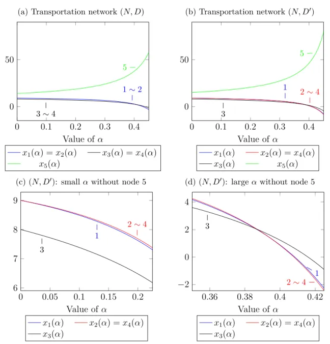
Generalized distance sums with various values of 𝛼 are given in Figure 3.
Figure 3: Generalized distance sums of Example 3 (a) Transportation network (𝑁, 𝐷)
0 0.1 0.2 0.3 0.4
0 50
1∼2
3∼4
5
Value of 𝛼
𝑥1(𝛼) =𝑥2(𝛼) 𝑥3(𝛼) = 𝑥4(𝛼) 𝑥5(𝛼)
(b) Transportation network (𝑁, 𝐷′)
0 0.1 0.2 0.3 0.4
0 50
1 2∼4
3
5
Value of 𝛼
𝑥1(𝛼) 𝑥2(𝛼) =𝑥4(𝛼) 𝑥3(𝛼) 𝑥5(𝛼) (c) (𝑁, 𝐷′): small𝛼 without node 5
0 0.05 0.1 0.15 0.2
6 7 8 9
1
2∼4
3
Value of 𝛼
𝑥1(𝛼) 𝑥2(𝛼) =𝑥4(𝛼) 𝑥3(𝛼)
(d) (𝑁, 𝐷′): large𝛼 without node 5
0.36 0.38 0.4 0.42
−2 0 2 4
1 2∼4 3
Value of 𝛼
𝑥1(𝛼) 𝑥2(𝛼) = 𝑥4(𝛼) 𝑥3(𝛼)
Nodes 1 and 2 as well as 3 and 4 are symmetric in (𝑁, 𝐷), while 2 and 4 are symmetric in (𝑁, 𝐷′), they have the same generalized distance sum for any𝛼. Generalized distance sums monotonically decrease with the exception of node 5 (see Figures 3.aand 3.b, where the numbers on the curves indicate the corresponding node). According to Figure 3.d, it can be achieved by increasing 𝛼 that𝑥1(𝛼)< 𝑥3(𝛼) (node 3 is less accessible than node 1) both in (𝑁, 𝐷) and (𝑁, 𝐷′).
The aim was to demonstrate that node 1 is more accessible than node 2 in (𝑁, 𝐷′) since they have the same distance sum but the former is closer to node 3 than the latter, and node 3 seems to be more accessible than node 4 as they were symmetric in (𝑁, 𝐷) and 𝑑45 has increased. This relation holds if 𝛼 is not too large (see Figures 3.c and 3.d).
Some basic attributes of generalized distance sum are listed below.
Proposition 2. Generalized distance sum satisfies the following properties for any fixed
1. Existence and uniqueness: a unique vector of x(𝛼) exists;
2. Anonymity (𝐴𝑁 𝑂);
3. Homogeneity (𝐻𝑂𝑀): the relation
𝑥𝑖(𝛼)(𝑁, 𝐷)≤𝑥𝑖(𝛼)(𝑁, 𝐷)⇒𝑥𝑖(𝛼)(𝑁, 𝛽𝐷)≤𝑥𝑖(𝛼)(𝑁, 𝛽𝐷) holds for all 𝑖, 𝑗 ∈𝑁 and 𝛽 >0;2
4. Distance sum conservation: ∑︀𝑖∈𝑁𝑥𝑖(𝛼) =∑︀𝑖∈𝑁𝑑Σ𝑖 ; 5. Agreement: lim𝛼→0x(𝛼) =dΣ;
6. Flatness preservation (𝐹 𝑃): if 𝑑Σ𝑖 =𝑑Σ𝑗 for all 𝑖, 𝑗 ∈𝑁, then 𝑥𝑖(𝛼) =𝑥𝑗(𝛼) for all 𝑖, 𝑗 ∈𝑁.
Proof. We prove the statements above in the corresponding order.
1. Matrix (𝐼+𝛼𝐴) is positive definite if 0< 𝛼 <−1/min{𝜆 :𝜆𝐴=𝐴y}.
2. Generalized distance sum is invariant under isomorphism, it depends just on the structure of the transportation network and not on the labelling of the nodes.
3. The identities dΣ(𝑁, 𝛽𝐷) = 𝛽dΣ(𝑁, 𝐷) and 𝐴(𝑁, 𝛽𝐷) = 𝐴(𝑁, 𝐷) imply x(𝛼)(𝑁, 𝛽𝐷) =𝛽x(𝛼)(𝑁, 𝐷).
4. ∑︀𝑖∈𝑁𝑥𝑖(𝛼) = ∑︀𝑖∈𝑁 [︁𝑥𝑖(𝛼) +∑︀𝑗∈𝑁𝑎𝑖𝑗𝑥𝑗(𝛼)]︁ = ∑︀𝑖∈𝑁𝑑Σ𝑖 since ∑︀𝑖∈𝑁𝑎𝑖𝑗 = 0 for all 𝑗 ∈𝑁.
5. lim𝛼→0𝛼𝐴x(𝛼) =0.
6. 𝑥𝑖(𝛼) = 𝑑Σ𝑖 satisfies (𝐼+𝛼𝐴)x(𝛼) =dΣ in the case of 𝑑Σ𝑖 =𝑑Σ𝑗 for all 𝑖, 𝑗 ∈𝑁.
Regarding𝐴𝑁 𝑂, it remains an interesting question whether the opposite of symmetry is valid, i.e., two nodes have the same generalized distance sum for any 𝛼 >0 only if they are symmetric.
Homogeneity means that the accessibility ranking is invariant under the multiplication of all distances by a positive scalar (i.e. the choice of measurement scale).
The name of this accessibility index comes from the property distance sum conservation:
it can be interpreted as a way to redistribute the sum of distances among the nodes.
According to agreement, its limit is distance sum.
𝐹 𝑃 requires that generalized distance sum results in a tied accessibility between any nodes if distance sum also gives this result. The other direction (whether the flatness of generalized distance for a given 𝛼 implies the flatness of distance sum) requires further research.
Remark 5. Distance sum also satisfies the properties listed in Proposition 2 (with the obvious exception of agreement). Distance product does not meet distance sum conservation and flatness preservation.
Figure 4: Transportation network of Example 4
1
2
3
4
5
10
9 8
7 6
Triangle inequality is essential for an accessibility index satisfying 𝐹 𝑃.
Example 4. Consider the transportation network (𝑁, 𝐷)∈ 𝒩10 in Figure 4such that
∙ 𝑑𝑖𝑗 = 1 if and only if nodes 𝑖 and 𝑗 are connected;
∙ 𝑑𝑖𝑗 = 10 if and only if nodes 𝑖and 𝑗 are not connected.
Then𝑑Σ𝑖 = 3×1 + 6×10 = 63 for all𝑖∈𝑁, but nodes 5 and 6 seems to be more accessible than the others. It is the case until 𝑑𝑖𝑗 >2 in the case of not connected nodes 𝑖 and 𝑗 since then there exists more shortcuts for nodes 5 and 6 than for the others.
It can be seen (e.g. from Example3) that generalized distance sum is better able to distinguish the accessibility of nodes than distance sum. In other words, there are far less nodes of equal generalized distance sum than there are for standard distance sum. It may be important in some applications (Lindelauf et al., 2013).
3.2 Connection to domination preservation
Generalized distance sum was constructed in order to eliminate independence of distance distribution. Proposition 2shows that anonymity is preserved in the process. Now we turn to the third axiom in the characterization of distance sum by Theorem 1, and investigate whether the suggested accessibility index meets domination preservation.
Notation 5. min𝑘{𝑆} and max𝑘{𝑆} are the 𝑘th smallest and largest element of a set 𝑆, respectively.
Theorem 2. Generalized distance sum satisfies 𝐷𝑃 if 𝛼 <min
⎧
⎨
⎩
min2{︁𝑑Σ𝑖 :𝑖∈𝑁}︁
max{𝑥𝑖(𝛼) :𝑖∈𝑁}; min{︁𝑑Σ𝑖 :𝑖∈𝑁}︁
max{𝑑Σ𝑖 :𝑖∈𝑁}
⎫
⎬
⎭
.
Proof. Consider a transportation network (𝑁, 𝐷) ∈ 𝒩 and two distinct nodes 𝑖, 𝑗 ∈ 𝑁 such that 𝑑𝑖𝑘 ≤ 𝑑𝑗𝑘 for all 𝑘 ∈ 𝑁 ∖ {𝑖, 𝑗} with a strict inequality (<) for at least one 𝑘.
Then
𝑥𝑖(𝛼) =
⎛
⎝1−𝛼∑︁
𝑘̸=𝑖
𝑑𝑖𝑘 𝑑Σ𝑘
⎞
⎠
−1⎡
⎣
∑︁
𝑘̸=𝑖
𝑑𝑖𝑘
(︃
1−𝛼𝑥𝑘(𝛼) 𝑑Σ𝑖
)︃⎤
⎦ and
𝑥𝑗(𝛼) =
⎛
⎝1−𝛼∑︁
𝑘̸=𝑗
𝑑𝑗𝑘 𝑑Σ𝑘
⎞
⎠
−1⎡
⎣
∑︁
𝑘̸=𝑗
𝑑𝑗𝑘
(︃
1−𝛼𝑥𝑘(𝛼) 𝑑Σ𝑗
)︃⎤
⎦.
The following two conditions are sufficient for 𝑥𝑖(𝛼)< 𝑥𝑗(𝛼):
∙ 𝛼𝑥𝑘(𝛼)/𝑑Σ𝑗 < 1 for any 𝑘 ∈𝑁 ∖ {𝑖, 𝑗}, that is, 𝛼 < 𝑑Σ𝑗/𝑥𝑘(𝛼), which provides that the ’contribution’ of 𝑑𝑗𝑘 to𝑥𝑗(𝛼) is positive;
∙ 𝛼∑︀𝑘̸=𝑖𝑑𝑖𝑘/𝑑Σ𝑘 ≤ 𝛼∑︀𝑘̸=𝑗𝑑𝑗𝑘/𝑑Σ𝑘 ≤ 𝛼𝑑Σ𝑗/min{︁𝑑Σℓ :ℓ∈𝑁}︁ < 1, namely, 𝛼 <
min{︁𝑑Σℓ :ℓ∈𝑁}︁/𝑑Σ𝑗.
Note also that 𝑑Σ𝑗 ≥min2{︁𝑑Σℓ :ℓ ∈𝑁}︁.
Remark 6. According to the proof of Theorem 2, the condition 𝛼 <min{︁𝑑Σ𝑖 :𝑖∈𝑁}︁/max{𝑥𝑖(𝛼) :𝑖∈𝑁}
provides that the ’contribution’ of any distance to any node’s generalized distance sum is positive, therefore it is positive, too (look at Figure 3.d).
Remark 7. Due to the continuity of x(𝛼), min2{︁𝑑Σ𝑖 :𝑖∈𝑁}︁>min{︁𝑑Σ𝑖 :𝑖∈𝑁}︁ implies min2{︁𝑑Σ𝑖 :𝑖∈𝑁}︁
max{𝑥𝑖(𝛼) :𝑖∈𝑁} > min{︁𝑑Σ𝑖 :𝑖∈𝑁}︁
max{𝑑Σ𝑖 :𝑖∈𝑁},
for small 𝛼, so the second expression is effective for small𝛼. Nevertheless, usually the first expression limits the value of the parameter 𝛼.
In a certain sense, the result of Theorem2is not surprising because distance sum meets 𝐷𝑃 and x(𝛼) is ’close’ to it when 𝛼 is small.3 The main contribution is the calculation of a sufficient condition. It is not elegant since it depends on x(𝛼), which excludes to check the requirement before the calculation,. However, ex post check is not difficult.
Definition 15. Reasonable upper bound: Parameter 𝛼 is reasonable if it satisfies the condition of Theorem 2for a transportation network (𝑁, 𝐷)∈ 𝒩. The largest 𝛼 with this property is the reasonable upper bound of the parameter.
Notation 6. The reasonable upper bound of generalized distance sum’s parameter is ^𝛼.
Remark 8. Generalized degree satisfies 𝐷𝑃 for any reasonable 𝛼 >0.
It is analogous to the (dynamic) monotonicity of a preference aggregation method called generalized row sum (Chebotarev,1994, Property 13) as well as to the adding rank monotonicity of a centrality measure generalized degree (Csat´o, 2015).
Violation of domination preservation may be a problem in practice.
Example 5. Consider the transportation network (𝑁, 𝐷′)∈ 𝒩5 in Figure 2, where node 3 dominates node 1 since 𝑑3𝑘 ≤𝑑1𝑘 for𝑘 = 2,4 and 𝑑35 < 𝑑15. However,𝑥3(0.4)> 𝑥1(0.4) according to Figure 3.d.
Theorem 2gives the reasonable upper bound as ^𝛼≈0.2686 from 𝛼 < min2{︁𝑑Σ𝑖 :𝑖∈𝑁}︁
max{𝑥𝑖(𝛼) :𝑖∈𝑁}.
Here min{︁𝑑Σ𝑖 :𝑖∈𝑁}︁/max{︁𝑑Σ𝑖 :𝑖∈𝑁}︁= 8/15. However, Theorem 2 does not give a necessary condition for 𝐷𝑃 since, for example,𝑥3(0.36)< 𝑥1(0.36) in Figure 3.d.
3 There always exists an appropriately small𝛼satisfying the condition of Theorem2.
Instead of domination preservation, which is a kind of ’static’ axiom, one can focus on the ’dynamic’ monotonicity properties of accessibility indices, similarly to independence of distance distribution of independence or irrelevant distances. This direction is followed by Sabidussi (1966) orChien et al. (2004) in the case of centrality measures. Then a plausible condition is the following.
Definition 16. Positive responsiveness to distances (𝑃 𝑅𝐷): Let (𝑁, 𝐷) ∈ 𝒩𝑛 be a transportation network and 𝑖, 𝑗, 𝑘 ∈𝑁 be three distinct nodes. Let 𝑓 :𝒩𝑛 →R𝑛 be an accessibility index such that 𝑓𝑖(𝑁, 𝐷)≤𝑓𝑗(𝑁, 𝐷) and (𝑁, 𝐷′)∈ 𝒩𝑛 be a transportation network identical to (𝑁, 𝐷) except for 𝑑′𝑗𝑘 > 𝑑𝑗𝑘.
𝑓 is calledpositively responsive to distances if 𝑓𝑖(𝑁, 𝐷)< 𝑓𝑗(𝑁, 𝐷).
Property𝑃 𝑅𝐷 demand that the position of a node in the accessibility ranking does not improve after an increase in its distances to other nodes. It has strong links to dominance preservation.
Lemma 6. 𝐴𝑁 𝑂 and 𝑃 𝑅𝐷 implies 𝐷𝑃.
Proof. Consider a transportation network (𝑁, 𝐷) ∈ 𝒩 and two distinct nodes 𝑖, 𝑗 ∈ 𝑁 such that 𝑑𝑖𝑘 ≤ 𝑑𝑗𝑘 for all 𝑘 ∈ 𝑁 ∖ {𝑖, 𝑗} with a strict inequality (<) for at least one 𝑘.
Define transportation network (𝑁, 𝐷′), which is the same as (𝑁, 𝐷) except for𝑑𝑖𝑘 = 𝑑𝑗𝑘 for all𝑘 ∈𝑁∖{𝑖, 𝑗}. Anonymity provides that𝑓𝑖(𝑁, 𝐷) =𝑓𝑗(𝑁, 𝐷), so positive responsiveness to distances implies 𝑓𝑖(𝑁, 𝐷)< 𝑓𝑗(𝑁, 𝐷).
Lemma 7. Distance sum, distance sum without ties and distance product meet 𝑃 𝑅𝐷.
Remark 9. Analogously to Theorem 1, distance sum can be characterized by 𝐴𝑁 𝑂,𝐼𝐷𝐷 and 𝑃 𝑅𝐷. Their independence is shown by the same three accessibility indices distance sum without ties, inverse distance sum, and distance product.
Proposition 3. There exists an anonymous accessibility index preserving dominance, which is not positively responsive to distances.
Proof. It is enough to define a function which gives an accessibility ranking of the nodes.
Definition 17. Lexicographic eccentricity: node𝑖is more accessible than node𝑗 if and only if max{𝑑𝑖𝑘 :𝑘∈𝑁} < max{𝑑𝑗𝑘 :𝑘∈𝑁} or max𝑚{𝑑𝑖𝑘 :𝑘 ∈𝑁} < max𝑚{𝑑𝑗𝑘 :𝑘 ∈𝑁} and maxℓ{𝑑𝑖𝑘 :𝑘 ∈𝑁}= maxℓ{𝑑𝑗𝑘 :𝑘 ∈𝑁} for all ℓ = 1,2, . . . , 𝑚−1.
It is the same as eccentricity (Hage and Harary, 1995), however, ties are broken by a lexicographic application of its criteria. Lexicographic eccentricity satisfies 𝐴𝑁 𝑂 and𝐷𝑃, but it is not positively responsive to distances since some distances in certain intervals has no effect on the accessibility ranking.
Remark 10. Remark 9and Proposition 3 show a somewhat surprising feature of axioma- tizations. Distance sum can be characterized by the three independent axioms of 𝐴𝑁 𝑂, 𝐼𝐷𝐷 and 𝑃 𝑅𝐷 as well as by 𝐴𝑁 𝑂, 𝐼𝐷𝐷 and 𝐷𝑃. However, 𝐷𝑃 is implied by 𝐴𝑁 𝑂 and 𝑃 𝑅𝐷. Therefore the second result seems to be stronger (as 𝐷𝑃 is strictly weaker than the combination of 𝐴𝑁 𝑂 and 𝑃 𝑅𝐷) but it is by the first axiomatization.
It remains an open question to give a sufficient condition for generalized distance sum to satisfy 𝑃 𝑅𝐷.
3.3 Two detailed examples
In the previous discussion, generalized distance sum was only a ’tie-breaking rule’ of distance sum in the reasonable interval of the parameter 𝛼. Therefore, it remains to be seen whether the choice of a reasonable𝛼may lead to significant changes in the accessibility ranking. The following examples reveal some interesting features of the measure, too.
Figure 5: Accessibility in the Ralik chain (see Example 6) (a) The voyaging network graph
of Marshall Islands’ Ralik chain
Bikini
Rongelap
Wotho
Ujae
Kwajalein Lae
Lib
Namu Ailinglaplap
Namorik Jaluit
Ebon
(b) Generalized distance sums
0 0.05 0.1 0.15 0.2 0.25 0.3
15 20 25 30 35 40
Bikini
Rongelap
Wotho
Ujae
Lae Lib
Ailinglaplap Jaluit
𝛼^
Value of𝛼
Bikini Rongelap Wotho
Ujae Lae Lib
Ailinglaplap Namorik ∼Jaluit
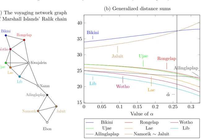
Example 6. The Marshall Islands in eastern Micronesia are divided into two atoll chains, one of them is Ralik. Figure 5.ashows the graph of the voyaging network of this island chain, constructed by Hage and Harary (1995). The distances of islands are measured by the shortest path between them. For instance, the distance of Bikini and Jaluit is 5 through Rongelap, Kwajalein, Namu and Ailinglaplap.
Note that Jaluit and Namorik are structurally equivalent in the network. Furthermore, Wotho dominates Rongelap and Ujae (it has extra links to Ujau and Lae, and to Bikini and Rongelap, respectively); Wotho and Rongelap dominate Bikini; Lae dominates Ujae;
Ailinglaplap, Namorik and Jaluit dominate Ebon.
Generalized distance sums are presented in Figure5.b. The reasonable upper bound is
^
𝛼 ≈0.2607, indicated by a (black) vertical line. However, the accessibility ranking does not violate 𝐷𝑃 for any 𝛼 in Figure 5.b.
Kwajalein (with a distance sum of 20) and Namu (21) are the first and second nodes in the accessibility ranking for any 𝛼. The difference between their generalized distance sums monotonically increases. Ebon (34) is ’obviously’ the least accessible node for any 𝛼.
These nodes do not appear in Figure5.b.
Compared to the distance sum, the following changes can be observed in the reasonable interval of 𝛼:
∙ The tie between Ailinglaplap and Wotho (25) is broken for Wotho. It makes sense since the nodes around Wotho have more links among them.
∙ The tie between Rongelap and Ujae (27) is broken for Ujae. It is justified by Ujae’s direct connection to Lae instead of Bikini as the former is more accessible than the latter.
∙ Lae (26) overtakes Ailinglaplap (25). The cause is that the network has essen- tially two components: the link between Ailinglaplap and Namu is a cut-edge, and the above part around Kwajalein (where Lae is located) is bigger and has more internal links.
Some other changes occur outside the reasonable interval of𝛼: Rongelap and Ujau overtake Ailinglaplap as well as Bikini overtakes Jaluit and Namorik. The reasoning applied for the case of Ailinglaplap and Lae is relevant here, too, and it is difficult to argue against these modifications of the ranking.
Example 6 verifies that the analysis of accessibility rankings should not automatically limit to the reasonable interval of parameter 𝛼, sometimes it is worth to consider values outside it. Remember that the condition of Theorem 2is only sufficient, but not necessary for dominance preservation.
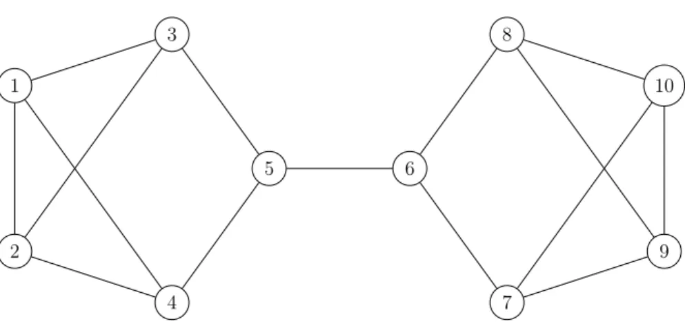
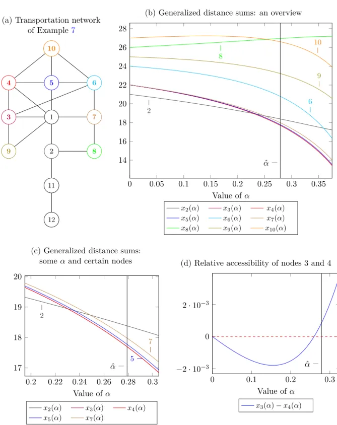
Example 7. Consider the network in Figure 6.a. The transportation network (𝑁, 𝐷)∈ 𝒩12 is such that the distances of nodes are measured by the shortest path between them.
For example, 𝑑1,12 = 3 due to the path (1,2)−(2,11)−(11,12).
Here node 1 dominates nodes 3, 8 and 9, node 2 dominates node 11, node 3 dominates node 9, node 5 dominates node 10 and node 11 dominates node 12.
Generalized distance sums are presented in Figure6.b. The reasonable upper bound is
^
𝛼 ≈0.279, indicated by a (black) vertical line. However, the accessibility ranking does not violate 𝐷𝑃 for any 𝛼 in Figure 6.b.
Node 1 (𝑑Σ1 = 17) is ’obviously’ the most accessible node for any𝛼. Nodes 11 (𝑑Σ11= 29) and 12 (𝑑Σ12= 37) are the last in the accessibility ranking for any reasonable value of 𝛼.
The difference between their generalized distance sums monotonically increases. These nodes do not appear in Figure 6.b.
Note that𝑥10(𝛼) is not monotonic, it has a maximum around 𝛼= 0.145.
Compared to the distance sum, the following changes can be observed in the reasonable interval of 𝛼:
∙ The tie between nodes 3, 4, 5 and 7 (𝑑Σ = 22) is broken in this order. Node 3 is more accessible than node 5 since node 9 is more accessible than node 10.
Node 3 is more accessible than node 7 since node 4 is more accessible than node 8 (and it has an extra link to node 9). Node 4 is more accessible than node 5 since node 3 is more accessible than node 6. Node 4 is more accessible than node 7 as its neighbours are more accessible. Node 5 is more accessible than node 7 since node 4 is more accessible than node 8 (and it has an extra link to node 10). The tie breaks are highlighted in Figure 6.c.
∙ The relation of nodes 3 and 4 (𝑑Σ = 22) is uncertain: both are connected to node 1, while node 5 is more accessible than node 6 (favouring node 4) and node 9 is more accessible than node 10 (favouring node 3). Node 3 benefits
Figure 6: Accessibility in Example 7
(a) Transportation network of Example 7
1
8 3
10
12
6
11
4 5
9 2
7
(b) Generalized distance sums: an overview
0 0.05 0.1 0.15 0.2 0.25 0.3 0.35
14 16 18 20 22 24 26 28
2
6 8
9 10
𝛼^
Value of𝛼
𝑥2(𝛼) 𝑥3(𝛼) 𝑥4(𝛼) 𝑥5(𝛼) 𝑥6(𝛼) 𝑥7(𝛼) 𝑥8(𝛼) 𝑥9(𝛼) 𝑥10(𝛼)
(c) Generalized distance sums:
some𝛼 and certain nodes
0.2 0.22 0.24 0.26 0.28 0.3 17
18 19 20
2
5 7
𝛼^
Value of𝛼
𝑥2(𝛼) 𝑥3(𝛼) 𝑥4(𝛼) 𝑥5(𝛼) 𝑥7(𝛼)
(d) Relative accessibility of nodes 3 and 4
0 0.1 0.2 0.3
−2·10−3 0 2·10−3
𝛼^
Value of𝛼 𝑥3(𝛼)−𝑥4(𝛼)
difference of generalized distance sums, red and purple lines are indistinguishable on Figures 6.b and 6.c.
∙ Node 10 (𝑑Σ10 = 27) overtakes node 8 (𝑑Σ8 = 26). It is more connected to the above ’component’ of the network. Furthermore, node 8 is closer to node 2, which gradually losses positions in the accessibility ranking.
∙ Nodes 3, 4, 5 and 7 (𝑑Σ = 22) overtake node 2 (𝑑Σ2 = 21). It is explained by the