3. k -hop based graph density and redundancy met- rics

(1)

Some k -hop based graph metrics and node ranking in wireless sensor networks ^*

Csaba Biró, Gábor Kusper

Eszterházy Károly University, Eger, Hungary biro.csaba@uni-eszterhazy.hu kusper.gabor@uni-eszterhazy.hu

Submitted: December 14, 2017 Accepted: September 13, 2018 Published online: February 27, 2019

Abstract

Node localization and ranking is an essential issue in wireless sensor networks (WSNs). We model WSNs by communication graphs. In our interpretation a communication graph can be directed, in case of heterogeneous sensor nodes, or undirected, in case of homogeneous sensor nodes, and must be strongly connected. There are many metrics to characterize networks, most of them are either global ones or local ones. The local ones consider only the immediate neighbors of the observed nodes. We are not aware of a metric which considers a subgraph, i.e., which is between global and local ones. So our main goal was to construct metrics that interpret the local properties of the nodes in a wider environment. For example, how dense the environment of the given node, or in which extent it can be relieved within its environment. In this article we introduce several novel𝑘-hop based density and redundancy metrics: Weighted Communication Graph Density (𝒲𝒞𝒢𝒟), Relative Communication Graph Density (ℛ𝒞𝒢𝒟), Weighted Relative Com- munication Graph Density (𝒲ℛ𝒞𝒢𝒟), Communication Graph Redundancy (𝒞𝒢ℛ), Weighted Communication Graph Redundancy (𝒲𝒞𝒢ℛ). We compare them to known graph metrics, and show that they can be used for node ranking.

Keywords: 𝑘-hop based graph metrics, communication graph density, com-

*This research was supported by the grant EFOP-3.6.1-16-2016-00001 “Complex improvement of research capacities and services at Eszterházy Károly University”

doi: 10.33039/ami.2018.09.002 http://ami.uni-eszterhazy.hu

19

(2)

munication graph redundancy, node ranking

MSC:68M07 68M17 68M12 68M15 68R10 05C05 05C12 05C40 05C82 90B10

1. Introduction

The modeling and analysis of complex networks is an important interdisciplinary field of science. The networks are mathematically related to graph theory. It is known that topology represents the properties of the whole network structure. A topology describes a real network (with constraints) and it can be converted to an undirected or directed graph. The common property of topological models is that they are usually calculated based on probabilities [2–4, 11]. The objects of the model can be matched by the vertices of the graph. Edges can be used to describe the relations between the objects. Graph-based modeling can be of two types: ad-hoc or measurement-based. On large wireless networks the traditional measurements based procedures can not be applied efficiently, but 𝑘-hop based approaches can be computed effectively also for large networks.

There are many graph-based metrics for modeling complex networks [9]. Topo- logical metrics commonly used on networks: number of nodes and edges, average degree, degree distribution, connectedness, diameter, number of independent paths.

Parameters for measuring the effectiveness of wireless networks: scope and coverage, scalability, expected transmission number, hop count(number of hops), power consumption / lifetime.

In graph theory, the density of a graph(𝒱;ℰ)can be calculated as _|𝒱|₍_|𝒱|−^|ℰ| ₁₎ [6].

Since the number of edges for a complete directed graph is|𝒱|(|𝒱| −1), the maximum density is 1. Clearly, the minimum density is 0 (for empty graphs). There are two different approaches [13, 16], but there is no strict distinction between sparse and dense graphs.

Distance-based metrics

The eccentricity of a node𝑢is defined as the longest hop count between the node 𝑢and any other node in the graph.

Centralization [8] is a general method for calculating a graph-level centrality score based on some node-level centrality metric. Centrality based metrics are the following ones: degree centrality (based on degree), closeness centrality (based on average distances), betweenness centrality (based on geodesics), eigenvector centrality(recursive: similar to page rank methods), eccentricity centrality. In the case of eccentricity centrality, we not use the reciprocal to assure that more central nodes have a higher value of eccentricity.

Connection-based metrics

The most basic connection-based metrics are the degree of a node, which is the number of edges to other nodes, and the degree distribution. The degree distribu-

(3)

tion𝑃(𝑘)of a graph is then defined to be the fraction of nodes in the network with degree𝑘. Thus if there are𝑛nodes in total in a graph and𝑛𝑘 of them have degree 𝑘, we have𝑃(𝑘) =𝑛𝑘/𝑛.

Clustering is a fundamental and important property of networks, just like degree and degree distribution. Clustering coefficient is the measurement that shows the opportunity of a graph to be divided into clusters. Clusters are disjoint subgraphs of the graph. A cluster usually should be a complete subgraph, so in this way it is similar to a clique, but a cluster may consists of one node, on the other hand a clique is a complete subgraph which contains always at least two nodes in case of a communication graph. The clustering coefficient can globally [12, 18] or locally [19]

characterize a graph. The global clustering coefficient is based on triplets of nodes.

The global clustering coefficient of a network, also known as transitivity𝑇, which is the ratio of the number of loops of length three and the number of paths of length two.Let𝑢be a vertex with𝑘degree and given by the proportion of𝑒edges between the 𝑣 within it is neighborhood 𝐺, then the Local clustering coefficient of 𝑢 in 𝐺 is given by 𝐶𝑢 = _𝑘(𝑘^2𝑒₋₁₎. Thus, 𝐶𝑢 measures the ratio of the number of edges between the neighbors of𝑢to the total possible number of such edges. The average clustering coefficient is the average of local clustering coefficients.

Wireless sensor networks

The ad hoc wireless sensor networks (WSN) are used widely(for example in military to observe environment). They have the advantage that they consist of sensors with low energy consumption, which can be deployed easily in a cheap way on such areas which are out-of-the-way. These sensors are the nodes of WSN. They are capable to process some limited information and to use wireless communication. A big effort is used to research how to deploy them in an optimal way to keep efficient energy consumption and communication. Although there are many WSN solutions, the deployment of a WSN is still an active research field [1].

One of the important property of an ad hoc wireless network is node density.

The dense layout makes the following properties available: high fault tolerance, high-coverage characteristics, but also cause some problems. The interference is high near to dense node areas, and there are a lot of collisions in case of message passing, which requires complicated operations for routing protocols, because of too many possible routes, routing needs lots of resources [5].

The aim of topology control techniques is to reduce the cost of the distributed algorithms interpreted on the network. The graph, which represents a network, has to be thinned because of cost-reduction by techniques like disconnection of nodes, removing links, changing scopes, etc., but the network-quality characteristics(like scalability, coverage, fault tolerance, etc.) must not fall below a required level. The overall aim is to create a scalable, fault-tolerant sparse topology, where the degree of the nodes are low, the maximum load is low, energy consumption is low and the paths are short. The following techniques are used to create an optimal topology:

reducing the scope of nodes, removing some nodes, introducing a dominating set

(4)

of nodes, clustering, and add some new nodes to gain all-all communication [15, 17].In multi-hop networks one hop is the unit of the path between source and destination. The hop count refers to the number of intermediate nodes through which data must pass between source and destination. Networks can be classified by the number of hops between source nodes, which measures their environment, and a sink node, which collects data. In a single-hop network there is only one (single) hop between the source nodes and the sink node. In a multi-hop network a sensor can also transmit data from the source to the sink because there are more than one hop from the source to the sink.

The rest of this article is organized as follows. In Section 2 we give some preliminary definitions, like communication graph. In Section 3 we introduce the new metrics, each of them are 𝑘-hop based. In Section 4 we compare existing metrics and the new ones. In section 5 we show how to use this metrics to rank nodes and Section 6 contains our conclusions.

2. Preliminaries

Given a randomly-deployed sensor network with homogeneous or heterogeneous nodes. Also given a mapping which sensor is able to communicate with which sensors directly. Accordingly, by communication graph we mean a weighted directed graph 𝒟 = (𝒮;ℰ𝒞,𝒲), where 𝒮 is the set of nodes, which represents the sensors, ℰ𝒞 ⊆ 𝒮 × 𝒮 is the set of edges, and𝒲 is the set of weights. An edge(𝑥𝑖, 𝑥𝑗)∈ ℰ𝒞

represents the possibility of messaging from node 𝑥𝑖 to 𝑥𝑗 in 𝒟, i.e., the sensor represented by 𝑥𝑗 is in the transmission range of 𝑥𝑖. The 𝒲^𝑖𝑗 denotes the communication cost of the(𝑥𝑖, 𝑥𝑗)message. In the case of homogeneous sensors the𝒟 graph is symmetric, accordingly𝒟= (𝒮;ℰ𝒞,𝒲)is equivalent to a simple weighted undirected graph 𝒢= (𝒮;ℰ𝒞,𝒲).

In case of an weighted undirected graph𝒢 = (𝒮;ℰ𝒞,𝒲) we define a clique as a subset of the node set 𝒞𝑙 ⊆ 𝒮, such that for every two nodes in𝒞𝑙, there exists an edge connecting the two. The weight of a𝒞𝑙 is the sum of the weight of their edges.

If our communication graph is directed, we define a clique as a subset of the node set 𝒞𝑙 ⊆ 𝒮, such that for every two nodes in 𝒞𝑙, there exists an edge from the first one to the second one, and from the second one back to the fists one.

The weight of the 𝒞𝑙 is defined as above, considering that𝒲^𝑖𝑗 and 𝒲^𝑗𝑖 are not necessarily equal. A maximal clique is a clique which is not a proper subset of any other clique. A𝑛-clique is a clique which contains exactly𝑛vertices.

In this paper we assume that the communication graph is strongly connected, the cost of communication between each node is constant(we do not use weights), and the network consists of homogeneous nodes. To test the new metrics we used our own representation [7] and SAT solver [10].

(5)

3. k -hop based graph density and redundancy met- rics

In this section we present some spanning tree and clique-based graph density metrics. With spanning tree-based metrics, we define graph density, whereas clique- based redundancy metrics mean the degree of relieving in our interpretation. We use the notion of 𝑘-hop environment of a node 𝑢, denoted by 𝒢^[𝑛](𝑢), which is a subgraph of graph 𝒢, which consists 𝑢and the nodes which can be reached from 𝑢from an path, which length is smaller or equal than𝑘, and which contains edges between these nodes from 𝒢. We compute local metrics for 𝑢 by computing a graph metrics for 𝒢^[𝑛](𝑢). The parameter 𝑘 should be a relatively small number because otherwise 𝒢^[𝑛](𝑢)could be the whole graph. The metrics over the𝑘-hop environment of a node can characterize the node more properly then considering merely the node itself. On the other hand these metrics characterize not only the node but its environment.

Taking into account the constraints mentioned in Section 2, the basic notations are:

∙ 𝑢: the candidate node;

∙ 𝑘: the number of hops;

∙ 𝒩,𝒱: the number of nodes and edges of graph𝒢;

∙ 𝒩^[𝑘](𝑢),𝒱^[𝑘](𝑢): the number of nodes and edges of graph𝒢^[𝑘](𝑢);

∙ 𝒞𝑙,ℳ: the set of maximum cliques of graph𝒢and the cardinality of this set;

∙ 𝒞𝑙^[𝑘](𝑢), ℳ^[𝑘](𝑢): the set of maximal cliques of graph𝒢^[𝑛](𝑢)and the cardinality of this set;

∙ 𝒯^[𝑘](𝑢),𝒯: the number of edges of the minimum cost spanning tree of graph 𝒢^[𝑘](𝑢) and 𝒢. Note, that in case of a communication graph we have that 𝒯 =𝒩 −1, regardless whether the graph is directed or undirected;

∙ 𝑠: the spreading factor, which is rather a technical value to enlarge small differences in the metrics, in this article we set𝑠= 2.71;

∙ 𝑐𝑠: the clique size, minimum value is 2.

3.1. Spanning tree-based metrics

Sanning tree-based approaches can be found in the wide area of network protocols.

For example, a known technique is Time-To-Live(TTL). It works as follows, routing methods try to find the best path for forwarding the collected data, the TTL mechanism is used to limit the number of hops to avoid over-overlapping of paths

(6)

and to balance the data load on the nodes and the energy consumption [14]. They use also small𝑘values.

We define graph density of the graphs𝒢 and𝒢^[𝑘](𝑢)as follows:

𝒢𝒟= 𝒱 𝒯 𝒢𝒟^[𝑘](𝑢) = 𝒱^[𝑘](𝑢)

𝒯^[𝑘](𝑢).

The graph density takes its maximum if the graph is complete. In case of undirected graphs the maximum is: ^𝒩_{2(𝒩 −1)}⁽^{𝒩 −}¹⁾ =^𝒩₂. In case of directed graphs the maximum is:

𝒩(𝒩 −1)

𝒩 −1 =𝒩. The graph density takes its maximum if the graph is a tree. In case of undirected graphs the minimum is: ^{𝒩 −}_{𝒩 −}¹₁ = 1, since the graph is a communication graph, i.e., it is strongly connected. If the graph is directed, then the minimum is:

2(𝒩 −1)

𝒩 −1 = 2, because of the same reason.

Communication and Weighted Communication Graph Density

We define the communication graph density of node𝑢in its𝑘-hop environment as follows:

𝒞𝒢𝒟^[𝑘](𝑢) =𝑠

𝒱[𝑘] (𝑢) 𝒯[𝑘] (𝑢).

The 𝒞𝒢𝒟^[𝑘](𝑢) can be used also as a local metric for a node, and computed quickly for all nodes and use to rank them.

We define the weighted communication graph density of node 𝑢 in its 𝑘-hop environment as follows:

𝒲𝒞𝒢𝒟^[𝑘](𝑢) =𝑠

𝒱[𝑘] (𝑢)

𝒯[𝑘] (𝑢)𝒩^[𝑘](𝑢) 𝒩 .

The𝒲𝒞𝒢𝒟^[𝑘](𝑢)is no longer a purely local metric, but takes into account the number of nodes in the𝑘-hop environment.

Relative Communication Graph Density

We define the relative communication graph density of node 𝑢 in its 𝑘-hop environment as follows:

ℛ𝒞𝒢𝒟^[𝑘](𝑢) =𝑠^𝒞𝒢𝒟

[𝑘] (𝑢) 𝒞𝒢𝒟 =𝑠^𝒱

[𝑘](𝑢)𝒯 𝒯[𝑘](𝑢)𝒱.

It maximizes its value when the𝑘-hop environment of𝑢, i.e., 𝒢^[𝑘](𝑢)is a complete graph and the rest of the graph is a tree, or consists of several trees.

The minimum is - vice versa - assumes that the 𝑘-hop environment of 𝑢is a tree and the rest of the graph is a complete graph.

If we consider the two extremes, i.e., if the communication graph is a complete graph or if it is a tree, interestingly enough, we get the same relative communication

(7)

graph density, which is𝑠. If the communication graph is a complete graph, then for any𝑘 >= 1and for any node𝑢we have that𝒢^[𝑘](𝑢)is equal to𝒢, so, _𝒯^𝒱^[𝑘][𝑘]^(𝑢)(𝑢) =_𝒯^𝒱, i.e., ^𝒱_𝒯^[𝑘][𝑘]^(𝑢)(𝑢)^𝒯𝒱 = 1. On the other hand, if the communication graph is a tree, then its communication graph density is a constant (1if the graph is undirected, 2if it is directed) for any 𝑛and𝑢, so again ^𝒱_𝒯^[𝑘][𝑘]^(𝑢)(𝑢)^𝒯𝒱 = 1.

We get the same result for the two extreme cases, because this metric shows the relative density of subgraph related to the whole graph. A tree has a very small density, and a complete graph has a very high density, but if we take a subgraph of a tree then it has the same density as the whole, and the same is true for a complete graph. So they have the same relative density.

This metric shows whether the𝑘-hop environment of a node is more dense as the whole graph, or has the same density, or it is less dense. This means that if

∙ ℛ𝒞𝒢𝒟^[𝑘](𝑢) =𝑠, then𝒢^[𝑘](𝑢)has the same cgd as𝒢;

∙ ℛ𝒞𝒢𝒟^[𝑘](𝑢)< 𝑠, then𝒢^[𝑘](𝑢)has smaller cgd than𝒢;

∙ ℛ𝒞𝒢𝒟^[𝑘](𝑢)> 𝑠, then𝒢^[𝑘](𝑢)has bigger cgd than𝒢;

where cgd means communication graph density.

Note, that this metric is computed by dividing a local property by a global one.

Weighted Relative Communication Graph Density

We define the weighted relative communication graph density of node𝑢in its𝑘-hop environment as follows:

𝒲ℛ𝒞𝒢𝒟^[𝑘](𝑢) =ℛ𝒞𝒢𝒟^[𝑘](𝑢)𝒩^[𝑘](𝑢) 𝒩 =𝑠

𝒱[𝑘] (𝑢)𝒯

𝒯[𝑘] (𝑢)𝒱𝒩^[𝑘](𝑢) 𝒩 .

Note, that this metric is computed as a multiplication of two numbers, which are both computed by dividing a local property by a global one, so we have (𝑙𝑜𝑐𝑎𝑙^′/𝑔𝑙𝑜𝑏𝑎𝑙^′)*(𝑙𝑜𝑐𝑎𝑙^′′/𝑔𝑙𝑜𝑏𝑎𝑙^′′).

This metric takes in consideration also how many nodes are in the 𝑛-hop environment of the node 𝑢. A node is more valuable if its 𝑘-hope environment is bigger.

3.2. Clique-based metrics

During the work of a WSN the topology of the network may change because some sensors may go wrong, or the transmission range can be less. If a node can be found in a dense (redundant) environment then it may happen more often that communication interference occurs and routing is more resource consuming; on the other hand, the environment itself is more fault tolerant. In a sparse environment routing is easier, communication interference is less frequent, but the environment is less fault tolerant. The aim of topology control techniques is to reduce the cost

(8)

of the distributed algorithms interpreted on the network. But the network-quality characteristics(like scalability, coverage, fault tolerance, etc.) must not fall below a required level. A clique is a complete subgraph, so they have high communication redundancy, on the other hand they allow high fault tolerance, results in high coverage, etc.

First of all we define the average clique size as follows:

𝒞ℒ= 1 ℳ

∑︁ℳ 𝑖=1

|𝒞𝑙𝑖|>=𝑐𝑠.

The average clique size is maximal, if the graph is complete. Its minimum is𝑐𝑠 if all maximal cliques have the size𝑐𝑠. It is not defined if there is no clique with size at least 𝑐𝑠. Its maximum is 𝒩 if the communication graph is complete, because then we have only one maximal clique, the graph itself. The clique problem, the problem of finding all maximal size cliques, is a well-known NP-complete problem.

It meas that is not feasible to find all maximal cliques in a large graph. So one can not use clique based metrics to guide topology control techniques, except if we work with relatively small graphs, like in the𝑘-hop environment of a node.

Clique size-based metrics

So we define the clique size-based communication graph redundancy of node 𝑢 within𝑘-hop environment as follows:

𝒞𝒢ℛ^𝑠𝑏^[𝑘](𝑢) = 1 ℳ^[𝑘](𝑢)

ℳ^[𝑘](𝑢)

∑︁

𝑖=1

⃒⃒

⃒𝒞𝑙^[𝑘](𝑢)𝑖

⃒⃒

⃒>=𝑐𝑠

It only shows the average clique size within 𝑘-hop environment of node𝑢, but it ignores the number of nodes within the 𝑘-hop environment.

We define weighted communication graph redundancy of node𝑢within𝑘-hop environment as follows:

𝒲𝒞𝒢ℛ^𝑠𝑏^[𝑘](𝑢) =𝒞𝒢ℛ^𝑠𝑏^[𝑘](𝑢)𝒩^[𝑘](𝑢) 𝒩 .

This metric uses also the number of nodesThis can be considered to be a local metric, because the computationally intensive tasks (find cliques) typically occur in a𝑘-hop environment.

Clique value-based metrics

Since a clique of size 4 is more valuable in a graph than6 in a graph with 100 nodes, we shall take into consideration the number of nodes in the graph, which is denoted by 𝒩, to compute the value of a clique. We also use the average clique size to normalize this value.

(9)

So we define the value of a clique as follows:

𝒞ℒ^𝑉 = |𝒞𝑙|>=𝑐𝑠

𝒩 𝑠^|𝒞

𝑙|>=𝑐𝑠 𝒞ℒ . We define also the average value of cliques as follows:

𝒞ℒ^𝑉 = 1 ℳ

∑︁ℳ 𝑖=1

|𝒞𝑙𝑖|>=𝑐𝑠

𝒩 𝑠^|𝒞^𝑙𝑖^𝒞ℒ^|>=𝑐𝑠

We define also the average value of cliques within the 𝑘-hop environment, also called clique value-based communication graph redundancy as follows:

𝒞𝒢ℛ^𝑣𝑏^[𝑘](𝑢) = 1

1 ℳ^[𝑘](𝑢)

∑︀ℳ^[𝑘](𝑢)

𝑖=1 |𝒞𝑙^[𝑘](𝑢)𝑖|>=𝑐𝑠

𝒩^[𝑘](𝑢) 𝑠

|𝒞𝑙[𝑘](𝑢)𝑖|>=𝑐𝑠 𝒞ℒ[𝑘] (𝑢)

.

This metric is the pair of𝒞ℒ^𝑉 in case of 𝒢^[𝑘](𝑢). This is a local metric, but this notion does not takes into consideration the number of nodes in the 𝑘-hop environment of 𝑢. Without reciprocal, the peripheral but relievable nodes are ranked in advance.

After considerating the number of nodes in the𝑘-hop and conversion we define weighted clique value-based communication graph redundancy as follows:

𝒲𝒞𝒢ℛ^𝑣𝑏^[𝑘](𝑢) = 1 𝒞𝒢ℛ^𝑣𝑏^[𝑘](𝑢)

𝒩^[𝑘](𝑢) 𝒩 =

= 1

ℳ^[𝑘](𝑢)

∑︁

𝑖=1

𝒩^[𝑘](𝑢)|𝒞𝑙^[𝑘](𝑢)𝑖|^>=𝑐𝑠

𝒩² 𝑠

|𝒞𝑙[𝑘](𝑢)𝑖|>=𝑐𝑠 𝒞ℒ[𝑘] (𝑢)

This metric is the pair of 𝒞ℒ^𝑉 in case of𝒢^[𝑘](𝑢).

4. Comparisons with other metrics

In this article we considered networks with 200-500 nodes at 15-40% densities. The 𝑘 value in each case is less than 3. An important constraint was that the largest 𝑘-hop environment must be smaller than the quarter of a complete graph.

For simulating and analyzing networks we used a self-developed Python tool based on NetworkX¹. For computing pairwise correlation of metrics we usedpan- das². Many metrics are only implemented for undirected graphs in NetworkX, therefore, the comparisons were done only on undirected graphs.

The results of the correlation analysis are presented in Table 1–3(average values of 1000 runs), shows some interesting phenomena and experience. The abbrevation c. means centrality.

1https://networkx.github.io

2https://pandas.pydata.org

(10)

4.1. 1-hop based environment

𝑘-hop based metrics

𝒲𝒞𝒢𝒟[𝑘] ℛ𝒞𝒢𝒟[𝑘] 𝒲ℛ𝒞𝒢𝒟[𝑘] 𝒲𝒞𝒢ℛ𝑠𝑏[𝑘] 𝒞𝒢ℛ𝑣𝑏[𝑘] 𝒲𝒞𝒢ℛ𝑣𝑏[𝑘]

Clustering coeff. 0,06 0,19 0,00 0,37 -0,17 0,14

Eccentricity -0,07 -0,21 -0,24 -0,15 -0,31 -0,21

Betweenness c. -0,04 -0,05 0,06 -0,12 0,22 -0,01

Degree c. 0,54 0,87 0,94 0,76 0,84 0,83

Closeness c. 0,05 0,23 0,28 0,17 0,37 0,23

Eigenvector c. 0,67 0,61 0,64 0,49 0,28 0,68

Table 1: Correlations with other metrics, where𝑘is1

It can be seen from the Table 1 that within 1-hop environment the defined metrics show their most significant correlation with degree centrality. The correlation is the strongest between𝒲ℛ𝒞𝒢𝒟and degree centrality, the correlation is over 90%. 𝒲𝒞𝒢𝒟, ℛ𝒞𝒢𝒟,𝒲ℛ𝒞𝒢𝒟 and𝒲𝒞𝒢ℛ^𝑣𝑏 metrics are also strongly correlated with the eigenvector centrality.

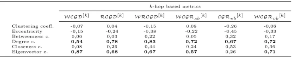
4.2. 2-hop based environment

Clustering coeff. -0,07 0,04 -0,15 0,08 -0,26 -0,06

Eccentricity -0,15 -0,24 -0,38 -0,22 -0,45 -0,33

Betweenness c. 0,06 0,03 0,22 0,05 0,32 0,17

Degree c. 0,54 0,78 0,83 0,72 0,67 0,72

Closeness c. 0,08 0,26 0,44 0,24 0,53 0,36

Eigenvector c. 0,87 0,68 0,67 0,57 0,26 0,71

It can be seen from the Table 2 that the defined metrics within 2-hop environment showed a weaker correlation with the degree centrality and stronger with the eigenvector centrality, since the degree of neighbors of the examined node also affects the density and redundancy of the environment. The strongest correlation with the degree centrality is still shown with𝒲ℛ𝒞𝒢𝒟, while with the eigenvector centrality correlats best with𝒲𝒞𝒢𝒟.

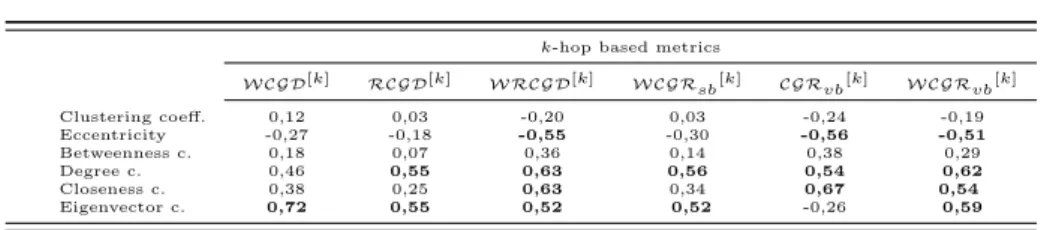
4.3. 3-hop based environment

The correlations in the 3-hop environment are shown in the Table 3. In general, the correlations with the degree centrality and the eigenvector centrality are no longer significant, the eccentricity and the closeness centraliy correlations are reinforced.

In the following, we will analyze in detail the relationship between the new and already known metrics.

(11)

Clustering coeff. 0,12 0,03 -0,20 0,03 -0,24 -0,19

Eccentricity -0,27 -0,18 -0,55 -0,30 -0,56 -0,51

Betweenness c. 0,18 0,07 0,36 0,14 0,38 0,29

Degree c. 0,46 0,55 0,63 0,56 0,54 0,62

Closeness c. 0,38 0,25 0,63 0,34 0,67 0,54

Eigenvector c. 0,72 0,55 0,52 0,52 -0,26 0,59

Weighted Communication Graph Density

The metric𝒲𝒞𝒢𝒟^[𝑘](𝑢) correlats strongly with eigenvector centrality. There is a not too strong but significant correlation with degree centrality also, and there is no relevant correlation with other metrics. If we want to characterize this metric on the basis of the above, then a high 𝒲𝒞𝒢𝒟^[𝑘](𝑢) value node has the following properties (in𝑘-hop environment, if𝑘= 3):

∙ average probability of high number of direct connections,

∙ high probability of high degree of neighbors,

∙ weak probability of central location.

Relative Communication Graph Density

The metric ℛ𝒞𝒢𝒟^[𝑘](𝑢)has average correlation with degree centrality and eigenvector centrality, weak but significant contact with closeness centrality, and there is no relevant correlation with other metrics. So a highℛ𝒞𝒢𝒟^[𝑘](𝑢)value node has the following properties (in𝑘-hop environment, if𝑘= 3):

∙ average probability of high degree of neighbors.

Weighted Relative Communication Graph Density

The metric𝒲ℛ𝒞𝒢𝒟^[𝑘](𝑢)has an average linear correlation with degree centrality, closeness centrality, and eigenvector centrality, and suggests a weak correlation with betweenness centrality, but with eccentricity shows an average but inverse correlation. So a high 𝒲ℛ𝒞𝒢𝒟^[𝑘](𝑢) value node has the following properties (in 𝑘-hop environment, if𝑘= 3):

∙ average probability of central location,

∙ average probability of high degree of neighbors,

∙ weak probability of high geodesic distance from any other node.

(12)

Weighted Communication Graph Redundancy(size-based)

The metric𝒲𝒞𝒢ℛ^𝑠𝑏^[𝑘](𝑢)has average correlation with degree centrality and eigenvector centrality. It suggests a weak but significant correlation with closeness centrality and inverse correlation with eccenticity. There is no relevant correlation with other metrics. So a high𝒲𝒞𝒢ℛ^[𝑘]𝑠𝑏(𝑢)value node has the following properties (in𝑘-hop environment, if𝑘= 3):

∙ weak probability of central location.

Communication Graph Redundancy (value-based)

The metric𝒞𝒢ℛ^[𝑘]𝑣𝑏(𝑢)has an average linear correlation with degree centrality and closeness centrality. It suggests a weak correlation with betweenness centrality.

It shows shows an average but inverse correlation with eccentricity. So a high 𝒞𝒢ℛ^[𝑘]𝑣𝑏(𝑢)value node has the following properties (in𝑘-hop environment, if𝑘= 3):

∙ weak probability of great geodesic distance from any other node.

Weighted Communication Graph Redundancy(value-based)

The metric 𝒲𝒞𝒢ℛ^[𝑘]𝑣𝑏(𝑢) has an average linear correlation with degree centrality, closeness centrality, and eigenvector centrality. It suggests a weak correlation with betweenness centrality, but with eccentricity shows an average but inverse correlation. So a high 𝒲𝒞𝒢ℛ^[𝑘]𝑣𝑏(𝑢)value node has the following properties (in 𝑘-hop environment, if𝑘= 3):

∙ weak probability of great geodesic distance from any other node.

(13)

5. Node ranking

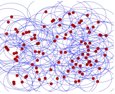
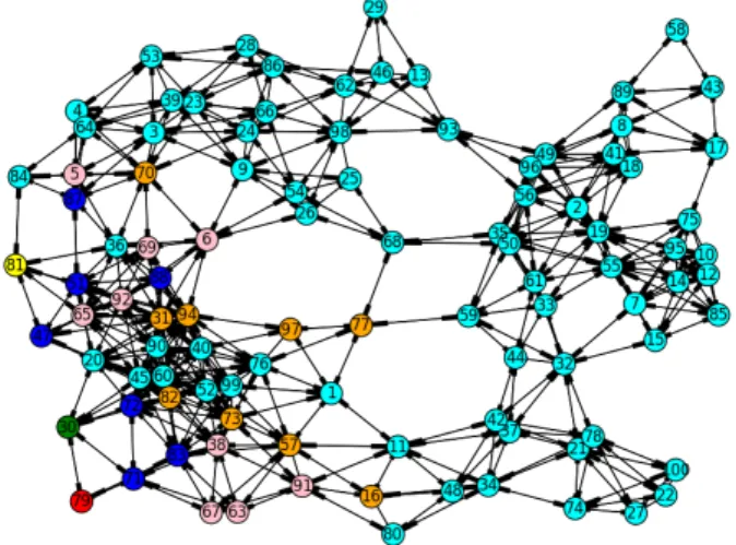
In this section we show how to use the different metrics to make node ranking(top 30 selection). The generated network (shown in Fig. 1 ) contains 100 randomly deployed and homogeneous sensor nodes (vertices) with 926 connections (edges).

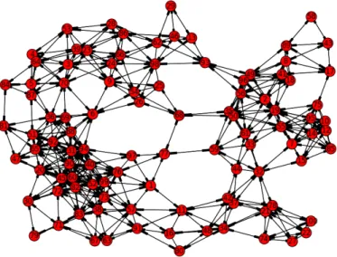
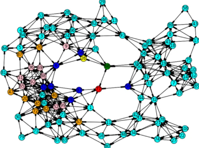
The density is 18.7%, the transmission range is55m, the area is300m×300m and the 𝑘-hop number is 3. The communication graph of the exemplary network are shown Fig. 2.

Figure 1: Randomly Deployed Sensor Network

Both the spanning tree and the clique based metrics show the denser environments of the network. Since this network consists of only 100 nodes it does not give a real picture of the metrics, but we can still see the tendencies.

Spanning tree-based metrics (density)

Figures 3–5 show how to use the spanning tree based metrics to make ranking nodes.

The task of all three metrics is to designate the densest environments. Based on the comparisons, the most significant feature of 𝒲𝒞𝒢𝒟is that the neighbors and the neighbors’ neighbors have a high degree. Figure 3 shows that the top 3 node and the at least 40% of the selected nodes are centrally located. The metricℛ𝒞𝒢𝒟 showed no significant correlation with the closeness centrality and eccentricity. In Figure 4 we can see that among the selected nodes there are only few nodes in central position. The metricℛ𝒞𝒢𝒟 primarily marks the nodes within the densest areas. The metric 𝒲𝒞𝒢𝒟 selects those nodes whose density is high within their

(14)

Figure 2: Communication Graph

𝑘-hop environment and centrally located. Figure 5 shows that the top 3 node and the at least 80% of the selected nodes are centrally located.

In these figures we use the following colour codes: top 1 rank node is red, top 2 is green, top 3 is yellow, top 4–10 are blue, top 11–20 are pink, top 21–30 are orange, the rest is cyan.

Figure 3 shows the top 30 ranked nodes based on theWeighted Communication Graph Densitymetric. In 3-hop environments, the highest weighted communication graph density has nodes 77, 68, and 26.

Figure 3: Weighted Communication Graph Density

(15)

Figure 4 shows the top30ranked nodes based on theRelative Communication Graph Density metric. In3-hop environments, the highest relative communication graph density has nodes 30, 79, and 71.

Figure 4: Relative Communication Graph Density

Figure 5 shows the top 30 ranked nodes based on theWeighted Relative Com- munication Graph Density metric. In 3-hop environments, the highest weighted relative communication graph density has nodes 68, 77, and 26.

Figure 5: Weighted Relative Communication Graph Density

(16)

Clique-based metrics (degree of relieving)

Figures 6–8 show how can we use the clique based metrics to make ranking nodes.

The task of all three metrics is to designate the degree of relieving nodes within their 𝑘-hop environment. Figure 6 shows node ranking created by 𝒲𝒞𝒢ℛ^𝑠𝑏. In case of𝒲𝒞𝒢ℛ^𝑠𝑏 only the size of cliques in the𝑘-hop environment of the examined node is relevant. 𝒲𝒞𝒢ℛ^𝑠𝑏 marks primarily the nodes within the densest areas, just likℛ𝒞𝒢𝒟. Figure 7 shows node ranking created by𝒲𝒞𝒢ℛ^𝑣𝑏. The significant difference between𝒲𝒞𝒢ℛ^𝑣𝑏and𝒲𝒞𝒢ℛ^𝑠𝑏is that𝒲𝒞𝒢ℛ^𝑣𝑏takes into consideration also the degree of neighbors. Figure 8 clearly shows that 𝒞𝒢ℛ^𝑣𝑏primarily focuses on centrally located nodes so the top 3 node and the at least 80% of the selected nodes are centrally located.

Figure 6 shows the top30ranked nodes based on theClique size-based Weighted Communication Graph Redundancy metric. In 3-hop environments, the most relieved nodes has nodes 79, 30, and 81.

Figure 6: Clique size-based Weighted Communication Graph Re- dundancy

Figure 7 shows the top 30 ranked nodes based on theClique value-based Com- munication Graph Redundancy metric. In 3-hop environments, the most relieved nodes has nodes 68, 77, and 26.

(17)

Figure 7: Clique value-based Communication Graph Redundancy

Figure 8 shows the top 30 ranked nodes based on theClique value-based Weight- ed Communication Graph Redundancy metric. In 3-hop environments, the most relieved nodes has nodes 77, 68, and 26.

Figure 8: Clique value-based Weighted Communication Graph Re- dundancy

These figures show that 1-1 densities and redundancy-based metrics similarly rank the nodes. Why? The first reason is that the two concepts are closely related, if the density is high, then the redundancy is high, too. However, if the test is performed with directed graphs, there will be significant differences, because if node𝑢can send a message to node𝑣, then𝑣may not be able to send a message to 𝑢, which means that high density does not mean necessarily also high redundancy.

(18)

6. Conclusions and Future work

In this paper we introduced several novel 𝑘-hop based density and redundancy metrics. We compared them to well-known graph metrics and we showed how can them be used for node ranking. Our primary goal was to define metrics that are able to rank nodes depending on their immediate environment within the whole network. Based on the results, we think that more sophisticated node ranking can be given using the new metrics. We primarily focused on modelling small heterogeneous networks. Metrics are defined so that they can be used also on networks where communication costs are different(weighted directed graphs). Our further goal is to investigate also such networks. An interesting questions is how to use these metrics to increase the efficiency of different(Tx range-based, hierarchical) topology control methods and how to use them in different hierarchical topological models (e.g. clustering, cluster head selection).

References

[1] I. F. Akyildiz,W. Su,Y. Sankarasubramaniam,E. Cayirci:A survey on sensor networks, IEEE Communications magazine 40.8 (2002), pp. 102–114,doi:10.1109/MCOM.2002.

1024422.

[2] R. Albert,A.-L. Barabási:Statistical mechanics of complex networks, Reviews of modern physics 74.1 (2002), p. 47.

[3] A.-L. Barabási,R. Albert,H. Jeong:Scale-free characteristics of random networks: the topology of the world-wide web, Physica A: statistical mechanics and its applications 281.1-4 (2000), pp. 69–77.

[4] S. Boccaletti,V. Latora,Y. Moreno,M. Chavez,D.-U. Hwang:Complex networks:

Structure and dynamics, Physics Reports 424.4 (2006), pp. 175–308,issn: 0370-1573,doi:

10.1016/j.physrep.2005.10.009.

[5] Bolic, Miodrag, Simplot-Ryl, David Stojmenovic, Ivan (eds.):RFID Systems - Re- search Trends and Challenges, New York: John Wiley & Sons, 2010, p. 576,isbn: 978-0-470- 74602-8,doi:10.1002/9780470665251.

[6] T. F. Coleman,J. J. Moré:Estimation of sparse Jacobian matrices and graph coloring blems, SIAM journal on Numerical Analysis 20.1 (1983), pp. 187–209.

[7] G. K. Csaba Biró:Equivalence of Strongly Connected Graphs and Black-and-White 2-SAT Problems, Miskolc Mathematical Notes 19.2 (2018), pp. 755–768,doi:10.18514/MMN.2018.

2140.

[8] L. C. Freeman: Centrality in social networks conceptual clarification, Social Networks (1978), p. 215,doi:10.1.1.227.9549.

[9] J. M. Hernández,P. Van Mieghem:Classification of graph metrics, Delft University of Technology: Mekelweg, The Netherlands (2011), pp. 1–20.

[10] G. Kusper,C. Biró,G. B. Iszály:SAT solving by CSFLOC, the next generation of full- length clause counting algorithms, in: 2018 IEEE International Conference on Future IoT Technologies (Future IoT), IEEE, 2018, pp. 1–9,doi:10.1109/FIOT.2018.8325589.

[11] A. Lesne:Complex networks: from graph theory to biology, Letters in Mathematical Physics 78.3 (2006), pp. 235–262,doi:10.1007/s11005-006-0123-1.

(19)

[12] R. D. Luce,A. D. Perry:A method of matrix analysis of group structure, Psychometrika 14.2 (June 1949), pp. 95–116,issn: 1860-0980,doi:10.1007/BF02289146,url:10.1007/

BF02289146.

[13] J. Nešetřil,P. O. De Mendez:First order properties on nowhere dense structures, The Journal of Symbolic Logic 75.3 (2010), pp. 868–887,doi:10.2178/jsl/1278682204.

[14] D. Rewadkar,M. P. Madhukar:An adaptive routing algorithm using dynamic TTL for data aggregation in Wireless Sensor Network, in: Second International Conference on Current Trends In Engineering and Technology-ICCTET 2014, IEEE, 2014, pp. 192–197, doi:10.1109/ICCTET.2014.6966286.

[15] P. Santi:Topology Control in Wireless Ad Hoc and Sensor Networks, ACM Computing Surveys 37.2 (2005), pp. 164–194,issn: 0360-0300,doi:10.1145/1089733.1089736.

[16] I. Streinu,L. Theran:Sparse hypergraphs and pebble game algorithms, European Journal of Combinatorics 30.8 (2009), Combinatorial Geometries and Applications: Oriented Ma- troids and Matroids, pp. 1944–1964,issn: 0195-6698,doi:10.1016/j.ejc.2008.12.018.

[17] Y. Wang:Topology Control for Wireless Sensor Networks, Springer - Wireless Sensor Net- works and Applications 148.2 (2008), pp. 113–147,issn: 1860-4862,doi:10.1007/978- 0- 387-49592-7.

[18] S. Wasserman,K. Faust:Social network analysis: Methods and applications, vol. 8, Cam- bridge university press, 1994.

[19] D. J. Watts, S. H. Strogatz:Collective dynamics of ’small-world’ networks, Nature 393.6684 (1998), pp. 440–442,issn: 00280836,doi:10.1038/30918.