A Time Petri Net Description of Membrane Systems with Priorities, Dissolution, and Promoters/Inhibitors
P´eter Batty´anyi, Gy¨orgy Vaszil?
Department of Computer Science, Faculty of Informatics University of Debrecen
Kassai ´ut 26, 4028 Debrecen, Hungary
{battyanyi.peter,vaszil.gyorgy}@inf.unideb.hu
Summary. We continue the investigations of the connection between membrane sys- tems and time Petri nets by extending simple symbol-object membrane systems with promoters/inhibitors, membrane dissolution and priority for rules. By constructing the simulating time Petri net, we retain one of the main characteristics of the Petri net model, namely, the firings of the transitions can take place in any order, there is no need to introduce maximal parallelism in the Petri net semantics. Instead, we substantially exploit the gain in computational strength obtained by the introduction of the timing feature for Petri nets.
1 Introduction
Several models have emerged in the past decades to model distributed systems with interactive, parallel components. One of them was developed by C.A. Petri [6], and since then the Petri nets have become the underlying system of a vast field of research with a considerable practical interest on the other hand. The theory of membrane systems was invented by Gh. P˘aun [4], and it has proved to be a very convenient and many-sided model of distributed systems with concurrent processes. Here we continue the investigations concerning the relationship of these two computational models.
Place/transition Petri nets are bipartite graphs, the conditions of the events of a distributed system are represented by places and directed arcs connect the places to the transitions, that model the events. The conditions for the events are expressed by tokens, an event can take place, i.e., a transition can fire, if there are enough tokens in the places at the ends of the incoming arcs of a transition. These places are called preconditions. The outgoing edges of a transition represent the
?Gy. Vaszil was supported by grant K 120558 of the National Research, Development and Innovation Office of Hungary (NKFIH), financed under the K 16 funding scheme.
postcondition of the events. Firing of a transition means removing tokens from the preconditions and adding them to the postconditions. The number of tokens moved in this way are prescribed by the multiplicities of the incoming and outgoing arcs.
In some cases the original place/transition model has turned out not to be satisfactory, for example, we are not able to model systems where a certain order of events must be taken into account. In order to deal with this difficulty, various extensions of the Petri net model have appeared. In this paper we deal with the time Petri net model developed by P.M. Merlin [3]. In this model, time intervals are associated to transitions. The local time observed from a transition can be modified by the Petri net state transition rules, and a transition can fire only if its observed time lies in the interval assigned to the transition by the construction of the model. In this way, the computational power of Petri nets is increased: the time Petri net model is Turing complete in contrast with the original state/transition Petri net.
Membrane systems are models of distributed, synchronized computational sys- tems ordered in a tree-like structure. The building blocks are compartments, which contain multisets of objects. The multisets evolve in each compartment in a paral- lel manner, and the compartments, in each computational step, wait for the others to finish their computation, hence the system acts in a synchronized manner. In every computational step, the multisets in the compartments evolve in a maximal parallel manner, this means that, in each step, as many rules of the compartment are applied simultaneously as possible.
In this paper we continue the research on the connection between time Petri nets and membrane systems initiated in [1]. We extend the basic construction of the time Petri net simulating a symbol object membrane system developed in [1] in order to represent some more membrane computational tools like pro- moters/inhibitors, membrane dissolution and priority of rules. One of the main features of our construction is that the unsynchronized characteristics of Petri nets is retained when a Petri net equivalent of a membrane system is presented.
That is, unlike the construction in [2] (and unlike the constructions in many other Petri net descriptions of membrane systems), we do not stipulate that the Petri nets should perform their computational steps in a maximal parallel manner, the attached time intervals provide the synchronization in the corresponding Petri nets. Similarly, there will be no need to introduce any other “special features”
(beside the feature of time) to be able to capture the effect of priorities, the use of promoters/inhibitors, or membrane dissolution.
2 Membrane Systems
Membrane systems are computational models operating on multisets. A finite mul- tiset over an alphabet O is a mapping M : O → N, where N is the set of non- negative integers. The number M(a) fora ∈ O is called the multiplicity of a in
M. We write that M1 ⊆M2 if for all a∈O, M1(a)≤M2(a). The union or sum of two multisets overO is defined as (M1+M2)(a) =M1(a) +M2(a), while the difference is defined forM2⊆M1as (M1−M2)(a) =M1(a)−M2(a) for alla∈O.
The set of all finite multisets over an alphabetOis denoted byM(O); the empty multiset is denoted by∅.
The notation N>0 stands for the set of positive integers, while Q and Q≥0
denotes the set of rational numbers and non-negative rational numbers andRand R≥0 the set of real numbers and non-negative real numbers, respectively.
We define the notion of the basic symbol-object membrane system [5] together with the additional features discussed in Section 5. A membrane system (or P sys- tem) is a tree-like structure of hierarchically arranged membranes. The outermost membrane is usually called the skin membrane. The membranes are labeled by natural numbers {1, . . . , n}, and we use the notation mi for a membrane labeled by i. Each membrane, except for theskin membrane, has its parent membrane.
We use µ for representing the structure of the membrane system itself, in fact, the structure itself can be given as a balanced string of left and right brackets indexed by their labels. For example, µ= [skin[1[2]2[3]3[4]4]skin. Here, the skin membrane has two submembranes, while region 1 also contains two embedded re- gions. Abusing the notation, µ(i) =k can also mean that the parent of the i-th region is regionk.
The regions contain multisets over a finite alphabet O. The contents of the regions of a P system evolve through rules associated with the regions. The rules constitute the micro steps of the computations. They are applied in a maximal par- allel manner. A computational step is the macro step of the process: it ends when each of the regions have finished their computations. A computational sequence is a sequence of computational steps.
Here we make the assumption that the computational steps in the regions consist of two phases: first the rule application phase produces from the objects on the left-hand sides of the rules the labeled objects on the right-hand sides (the labels of the labeled objects describe the way they should be moved between the regions: stay where they are, move to the parent region, or move into one of the children regions); then we have the communication phase when the labels are removed and all the objects are transported to the regions indicated by their labels. The P system gives a result when it halts, i.e., when no more rules can be applied in any of the regions. The result is a number or a tuple of natural numbers counting certain objects in the membrane designated as the output membrane.
AP system of degree n≥1 is Π = (O, µ, w1, . . . , wn, R1, . . . , Rn) where O is an alphabet of objects, µis a membrane structure ofn membranes,wi ∈ M(O) with 1≤i≤nare the initial contents of the nregions, Ri with (1≤i≤n) are the sets of evolution rules associated with the regions; they are of the formu→v, whereu∈ M(O) andv∈ M(O×tar), andtar={here, out} ∪ {inj|1≤j≤n}.
Unless stated otherwise, we consider then-th membrane as the output mem- brane. A configuration is the sequenceW = (w1, . . . , wn), wherewk is the multiset contained by membrane mk (1 ≤k ≤n). For a rule r: u→ v ∈Ri, we denote
bylhs(r) andrhs(r) the left-hand side and the right-hand side ofr, respectively (uand v, for the rule u→v). By the application of a rule u→v ∈Ri we mean the process of removing the elements of u from the multiset wi and extending wi with the labeled elements, which are called messages. As a result, during a computational step, a region can contain both elements of O and messages. An intermediate configuration is ann-tuple of multisets over O∪(O×tar). We say that W is aproper configuration, ifwi∈ M(O) for each of its regionswi.
The communication phase means that the elements coming from the right-hand sides of the rules of region i should be added to the regions as specified by the target indicators associated with them. If the right-hand side of a rulercontains a pair (a, here)∈O×tar, thena∈O is added to regioni, the region where the rule is applied. If it contains (a, out)∈O×tar, thenais added to the parent region of regioni. If it contains (a, inj)∈O×tar, thenais added to the contents of region j. In the latter case,µ(j) =iholds.
Given a (proper) configurationW, we obtain a new (proper) configurationW0 by executing the two phases of the transformations determined by the maximal parallel sets of rules chosen for each compartment of the membrane system. We call this a computational step, and denote it byW ⇒W0.
We might consider additional features being present in the membrane system.
First of all, we can add promoters and inhibitors to the rules. These are multisets of objects that regulate the rule applications in a way that the promoter z∈O∗ assigned to the rule r prescribes thatz must be present in the region where the rule is applied, while the inhibitor ¬z withz ∈ O∗ prevents the rule from being applied ifz is present in the region.
Second, we deal with the so-called membrane dissolution. The set of objects is extended with an additional elementδthat can appear on the right-hand sides of the rules. Ifδappears in a rulerwhich is applied in thei-th region for somei, then the communication phase is executed as before and, as the result of the presence of δ in region i, the region together with its set of rules Ri disappears from the P system. This means that the elements of region i(exceptδ, which disappears) are passed over to the region containingi(the parent region) and the rules inRi are not applied anymore. Note that the outermost region (theskinregion) cannot dissolve.
Finally, we consider a priority relation among rules. That is, we consider a partial order relation (an antisymmetric and transitive relation)ρi on the setRi for each 1 ≤i ≤n. We say thatr0 has priority over r, or r0 has higher priority than r, if (r0, r)∈ρi. In this case, if bothr0 andr were applicable in a maximal parallel step, thenris suppressed, that is, not allowed to be applied.
In Section 5 we show that all these features can be smoothly modeled by time Petri nets. The advantage of using time Petri nets instead of the Petri net models mostly applied in the literature (see e.g. [2]) is the fact that the usual order of the firings of the transitions is preserved: we do not inflict any additional firing condition on the transitions of the Petri nets (like the requirement that the
transitions fired in a computational step should constitute a maximal multiset of fireable transitions).
3 Time Petri Nets
In this section, following the definitions in [7] we define time Petri nets- a model rendering time intervals to transitions along the concept of Merlin [3]. First of all we define the underlying place/transition Petri nets, and then extend this model to the timed version.
APetri netis a tupleU = (P, T, F, V, m0) such that
1. P,T,F are finite, whereP∩T =∅,P∪T 6=∅ andF⊆(P×T)∪(T×P), 2. V :F →N>0,
3. m0:P →N.
The elements of P and T are called places and transitions, respectively. The el- ements of T are the arcs, and F is the flow relation of U. The function V is the multiplicity (weight) of the arcs, and m0 is the initial marking. In general, a marking is a function m:P →N. We may occasionally omit the initial marking and simply refer to a Petri net as the tuple U = (P, T, F, V). We stipulate that for every transition t ∈ T, there is a place p∈ P such that f = (p, t) ∈ F and V(f)6= 0.
Letx∈P∪T. The pre- and post-sets ofx, denoted by•xandx•respectively, are defined as•x={y|(y, x)∈F}andx•={y|(x, y)∈F}.
For each transitiont∈T, we define two markings,t−, t+:P →Nas follows:
t−(p) =
V(p, t), if (p, t)∈F,
0 otherwise, t+(p) =
V(t, p), if (t, p)∈F, 0 otherwise. A transitiont∈T is said to be enabled ift−(p)≤m(p) for all p∈•t.
Applying the notationMt(p) =t+(p)−t−(p) for p∈P, we define the firing of a Petri net. Let U = (P, T, F, V, m0) be a Petri net, and m be a marking in U. A transition t ∈T can fire in m (notation: m −→t ) if t is enabled in m.
After the firing of t, the Petri net obtains the new marking m0 : P → N with m0(p) =m(p)+Mt(p) for all p∈P. Notation:m−→tm0.
We obtain time Petri nets if we add time assigned to transitions of the Petri net. Intuitively, the time associated with a transition denote the last time when the transition was fired. We are considering only bounded time intervals. We present the definitions from [7], see also [8] for more information.
Definition 1.([7]) A time Petri net is a 6-tupleN = (P, T, F, V, m0, I)such that 1. the skeleton ofN given byS(N) = (P, T, F, V, m0)is a Petri net, and
2.I: T →Q×Q is a function assigning a rational interval to each transition, that is, for eacht∈T andI(t) = (I(t)1, I(t)2)we have that0≤I(t)1≤I(t)2.
We call I(t)1 andI(t)2 the earliest and the latest firing times belonging to t, and denote them byef t(t)andlf t(t), respectively.
Given a time Petri netsN = (P, T, F, V, m0, I), a functionm:P →Nis called ap-marking ofN. Note that talking about ap-marking ofNis the same as talking about a marking ofS(N).
Let N = (P, T, F, V, mo, I) be a time Petri net, m : P → N a p-marking in N, andhbe a function called a transition marking (ort-marking) inN,h:T → R≥0∪ {#}. A state in N is a pairu= (m, h) such that the two markingsm and hsatisfy the following properties: for allt∈T,
1. if t is not enabled in m (that is, if t−(p) > m(p) for some p ∈ •t), then h(t) = #,
2. iftis enabled inm(that is, ift−(p)≤m(p) for allp∈•t), thenh(t)∈Rwith h(t)≤lf t(t)).
The initial state is the pairu0= (m0, h0), wherem0 is the initial marking and for allt∈T,
h0(t) =
0, ift−(p)≤m0(p) for allp∈•t,
#, otherwise.
A transitiont∈T is ready to fire in stateu= (m, h) (denoted byu−→t) ift is enabled andef t(t)≤h(t).
We define the result of the firing for a transition that is ready to fire. Lett∈T be a transition and u = (m, h) be a state such that u −→t. Then the state u0 resulting after the firing of t denoted by u −→t u0 is a new state u0 = (m0, h0), such that m0(p) =m(p) +4t(p) for all p∈P. Now, for all transitions s∈T, we have
h0(s) =
h(s),ifs−(p)≤m(p), s−(p)≤m0(p) for allp∈•s, 0, ifs−(p)> m(p) for somep∈•s, but
s−(p)≤m0(p) for allp∈•s,
#, ifs−(p)> m0(p) for somep∈•s.
Hence, the firing of a transition changes not only the p-marking of the Petri net, but also the time values corresponding to the transitions. If a transitions∈T which was enabled before the firing oft remains enabled after the firing, then the valueh(s) remains the same, even ifsistitself. If ans∈T is newly enabled with the firing of transition t, then we set h(s) = 0. Finally, if s is not enabled after firing of transitiont, thenh(s) = #.
Observe that we ensure that a rule can be chosen more than once in a maximal parallel step that we allow transitions to be fired several times in a row: iftis fired resulting in the new p-marking m0 and t−(p) ≤m0(p) holds for allp∈ •t, then h(t) remains the same.
Besides the firing of a transition there is another possibility for a state to alter, and this is the time delay step. Letu= (m, h) be a state of a time Petri net, and τ ∈ R≥0. Then, the elapsing of time with τ is possible for the state u(denoted u−→τ) if for allt ∈ T, h(t) 6= # we haveh(t) +τ ≤lf t(t). Then the state u0,
namely the result of the elapsing of time byτ denoted byu−→τ u0 is defined as u0= (m0, h0), where m=m0 and
h0(t) =
h(t) +τ, ifh(t)6= #,
# otherwise.
Note that definitions ensure that we are not able to skip a transition when it is enabled: a transition cannot be disabled by a time jump. This kind of semantics is called the strong semantics in the literature [8].
We remark that classic Petri nets can be obviously obtained by havingh(t) = [0,0] for every transition, and no time delay step is ever made.
4 Connecting Petri Nets and Membrane Systems
First of all, we introduce the time Petri net model constructed in [1], which serves as our starting point in the constructions below. Our model relies on the corre- spondence between Petri nets and membrane systems described in [2], with the additional property that we do not require that our Petri net model should operate in a maximal parallel manner. In general, both by membrane systems and by Petri nets, a computational step can be considered as a multiset of rules or as a multiset of transitions, respectively. In the case of Petri nets, an application of a multiset of transitions is maximal parallel, if augmenting the multiset by any other transition results in a multiset of transitions that cannot be fired simultaneously in that con- figuration. In the case of membrane systems, maximal parallel execution means that, if we consider any membranemk, no rule ofmk can be added to our multiset of rules such that the remaining multiset still forms a multiset of executable rules inmk. In our construction, the fireable transitions of the simulating Petri nets can be executed in any order, we do not impose a restriction on the computational sequence of the Petri nets. This involves that we have made an essential use of the time feature, since the original place/transition Petri net model is not Turing complete, unlike the majority of the symbol object membrane systems.
We remark that, similarly to membrane systems, Petri nets can also be con- sidered as computational devices, which means that, if we start from an initial configuration such that an input is represented by the tokens contained by some designated places, then, when the computation halts, the content of the output places provide the result of the computation. Depending on the construction, the result can either be a number, or a tuple. The following statement is a reformu- lation of Theorem 4.2 in [1]. We present the proof with details here, since the subsequent Petri nets in the next section build upon this construction.
Theorem 1.([1]) Let Π = (O, µ, w1, . . . , wn, R1, . . . , Rn) be a membrane system without priorities, membrane dissolution and promoters/inhibitors.
Then there is a time Petri netN= (P, T, F, V, m0, I)such thatN halts if and only ifΠ halts and, if they halt, then they provide the same result.
Proof. The proof is a reinterpretation of that of Theorem 1 in [1]. We elabo- rate the construction again in order to keep our presentation self-contained. Let Π = (O, µ, w1, . . . , wn, R1, . . . , Rn) be a membrane system and let
N = (P, T, F, V, m0, I) be the corresponding Petri net. We define N so that a computational step ofΠ is simulated by two subnets ofN. The two subnets cor- respond to the two computational phases of a computational step of a membrane system, namely, the rule application and the communication phases. In our Petri net model, the tokens in the places P0 =O× {1, . . . , n} stand for the objects in the various compartments, while the tokens of the places ¯P0 = ¯O× {1, . . . , n}, where ¯O={¯a|a∈O}, represent the messages obtained in the course of the rule applications. Let us see the construction in detail.
• P =P0∪P¯0∪ {initapp, initcom, sem, enabld}, whereP0=O× {1, . . . , n} and P¯0= ¯O× {1, . . . , n}. Letm0(p) =wj(a) for every placep= (a, j)∈P0. Intuitively, the relation|p|=t, wherep= (a, i)∈O× {1, . . . , n}, means that there are as many astobjectsa∈Oin compartmentmi. In other words,wi(a) =t. On the other hand, the equality |¯p|=s, where ¯p= (¯b, j)∈O¯× {1, . . . , n}, expresses the fact that there arescopies of objectbthat will enter into membranemjat the end of the computational step. The placesinitcom, initapp, sem, enabld are places enabling the synchronization of the Petri net model.
• T =T0∪T0∗∪T#∪ {tapp, tcom, t1sem, t2sem}, where the transitions are defined as follows.
Let ri,j ∈ Ri, where 1 ≤ j ≤ |Ri| and 1 ≤ i ≤ n, be a rule in mi. Then the transitionti,j ∈T0 corresponds tori,j∈Ri. Let us define the arcs associated with ti,j for a fixediandj together with their multiplicities.
- Assume ti,j ∈T0, where 1 ≤i ≤nand 1 ≤j ≤ |Ri|. Thenp= (a, i)∈•ti,j
if and only ifa∈lhs(ri,j), and ¯p= (¯b, k)∈t•i,j if and only if either (b, ink)∈ rhs(ri,j), that is, mi is the parent region of mk, or (b, out)∈rhs(ri,j), where regionk is the parent region ofi, or k=j and (b, here)∈rhs(ri,j).
In addition,enabld∈•ti,j∩t•i,j (1≤i≤n,1≤j≤ |Ri|).
Regarding the weights of the arcs, letp = (a, i) and f = (p, ti,j)∈ F. Then the weight of f is the multiplicity of a ∈ O on the left-hand side of ri,j, namely,V(f) =lhs(ri,j)(a); furthermore, for ¯p= (¯b, k) and f = (ti,j,p)¯ ∈F, the weight of f is V(f) = rhs(ri,j)(b, ink) if region k is a child region of i, V(f) = rhs(ri,j)(b, out) if region k is the parent region of i, or V(f) = rhs(ri,j)(b, here) for k =j. Additionally, iff = (ti,j, enabld), thenV(f) = 1 (1≤i≤n,1≤j≤ |Ri|).
The transitions inT# are in charge with the correct simulation of a maximal parallel step: they fire only if there are any enabled rules in any of the regions.
Their inputs are the same as those of the elements ofT0, only their outputs differ, since they should not give rise to a change in the original distribution of the tokens before the computational step takes place.
- Letri,j∈Ri, where 1≤j ≤ |Ri|, 1≤i≤n; thent#i,j∈T# is the transition checking the applicability of ri,j. Let p= (a, i)∈ P0 and let t#i,j ∈T#; then p∈ •(t#i,j) and initapp ∈ •t#i,j and enabld ∈ (t#i,j)• and p∈ (t#i,j)•. In words, for a fixediandj,t#i,j expects as many tokens from its outgoing places as the number of distinct objects that is necessitated by an execution of the ruleri,j. In the meantime, a token arrives inenabld, which ensures the continuation of the simulation of the rule application phase. Thent#i,jgives back the tokens to the places inP0.
As regards the multiplicities, iff = (initapp, t#i,j) thenV(f) = 1, and if f = (t#i,j, enabld) then V(f) = 1; furthermore, if f = (p, t#i,j) or f = (t#i,j, p) where p= (a, i), thenV(f) =lhs(ri,j)(a).
The transitions in T0∗ ensure that tokens can flow back from ¯P0 to P0, thus representing the communication phase of the membrane computation.
- T0∗ = {sa,i | a ∈ O, 1 ≤ i ≤ n}. Let ¯p = (¯a, i) ∈ P¯0, then ¯p ∈ •sa,i and initcom ∈ •sa,i. Moreover, if p = (a, i), then p ∈ s•a,i and initcom ∈ s•a,i. Regarding the multiplicities, each arc has multiplicity 1.
The intervals belonging to the elements ofT =T0∪T0∗∪T#are [0,0]. The rest of the transitions are defined as follows.
- tappconnectsenabld, and hence the rule application part of the Petri net with the semaphore:enabld∈•tapp andsem∈t•app. Moreover, V(enabld, tapp) = 1 andV(tapp, sem) = 2 andI(tapp) = [1,1].
The role oftapp is to guarantee that a sequence of firings of transitions correctly simulates a maximal parallel application of membrane rules: every transition,ti,j
(1 ≤j ≤ |Ri|, 1 ≤ i ≤ n), corresponding to a rule execution can fire only if a token is found inenabld. On the other hand, if no transitionti,j can fire, then the transitiontappconnected only toenabldwill be activated after a time unit’s delay.
- tcom connectsinitcom, and the communication part of the Petri net with the semaphore: initcom ∈ •tcom and sem ∈ t•com. Moreover, V(initcom, tcom) = V(tcom, sem) = 1 andI(tcom) = [1,1].
The role of the semaphore is to make sure that the simulation of the rule application and the communication phases takes place in an alternating order.
This is achieved by the following machinery.
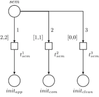
- Lett1sem and t2sem be transitions of the semaphore. Thensem ∈•(t1sem) and sem∈ •(t2sem); furthermore, initapp ∈(t1sem)• and initcom ∈ (t1sem)•. If f = (sem, t2sem), thenV(f) = 2. The weights of the other arcs are 1. In addition, I(t1sem) = [1,1] andI(t2sem) = [0,0].
To sum up the above construction: a computational step of a membrane system is split into a rule application and a communication phase, and those two phases are simulated separately and in an alternating order. The simulation of a phase finishes when no more rule applications are possible, hence we ensure that a maximal
parallel step is correctly simulated. When the rule application phase finishes its operation, 2 tokens are sent to the semaphore via tapp, and the simulation of the communication phase can immediately begin by forwarding the 2 tokens to initcom. Otherwise, when the communication phase finishes its operation, only 1 token is sent to the semaphore, so the rule application phase is initiated after a time unit’s wait. The structure of the various subnets are described in Figures 1, 2 and 3, respectively.
initapp enabld (a,1) (b,1)
tapp
[1,1] [0,0] t#1,1 [0,0] t1,1
sem (¯c,1) ( ¯d,2)
initapp enabld (a,1) (b,1)
tapp
[1,1] [0,0] t#1,1 [0,0] t1,1
sem (¯c,1) ( ¯d,2)
2
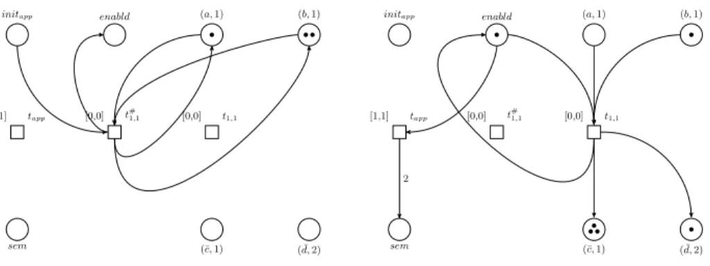
Fig. 1. Assumea, b2 ∈w(1) andr1,1 =ab→c3(d, in2), wherem2 is child ofm1. The figure shows the result of a single application of the rule in a split table: to the left is the subnet testing the applicability ofr1,1and to the right is the application of the rule itself.
The rule consumes anaand abin region 1 and three tokens are sent to the place (¯c,1), and one token to ( ¯d,2), in accordance with the fact that three objects of cshould be added to region 1, and one copy ofdshould be added to region 2 in the communication phase.
By this, we have simulated a membrane system with a time Petri net such that in the Petri net model no restriction on the transitions is made: the transitions
that are ready to fire can be fired in any order.
5 Extending the Correspondence to Membrane Systems with More Features
In this section we examine the possibility of extending our core model to Petri nets that are able to represent various properties of membrane systems, such as the presence of promoters/ inhibitors, membrane dissolution and priority among rules.
The obtained Petri nets each build upon the basic model defined in the previous section, so, in most of the cases, we restrict ourselves to emphasize only the new elements of the constructions by which the basic Petri net model is extended.
First we begin with discussing the case of promoters and inhibitors in the membrane system. Below we present a formal definition of promoters/inhibitors
sem (c,1) (d,2)
tcom [1,1]
1
sc,1
[0,0] [0,0] sd,2
initcom (¯c,1) ( ¯d,2)
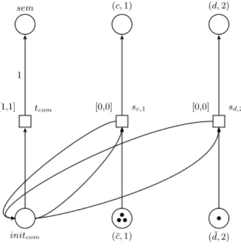
Fig. 2.The Petri net simulating the communication phase of a membrane computational step. When the simulation of a maximal parallel rule application step is finished, a token is given to the semaphoresem. The transitionssc,1, sd,2∈T0∗ensure the correct placement of the tokens corresponding to the messages.
sem
[1,1]
t1sem [0,0]
t2sem
initapp initcom
1 2
Fig. 3. The semaphore for the Petri net. When the simulation of the rule application phase of a computational step of the membrane system is complete, two tokens appear at sem, and then sent toinitcom, activating the simulation of the communication phase of the computational step. When the simulation of the communication phase is completed, one token appears at sem, which is then sent toinit0, activating the simulation of the rule application phase of a subsequent computational step.
in a form which is unusual, but technically well suitable for the presentation of the corresponding time Petri net model.
Definition 2.Let Π = (O, µ, w1, . . . , wn, R1, . . . , Rn,P) be a membrane system with promoters/inhibitors, where P(rj,i) ⊆ O∗×O∗, for every rj,i ∈ Ri. Then P(rj,i) = (ρj,i, τj,i)⊆O∗×O∗ is a promoter/inhibitor pair forrj. We denote the
pair (ρj,i, τj,i) by (promr, inhibr). Let R be a multiset of rules. A multiset R is applicable, if each of the following conditions fulfill.
1.lhs(rj,i)(a)· R(j, i)≤wi(a) (a∈O), 2.promr(a)≤wi(a) (r∈ R, a∈O), 3.wi(a)< inhibr(a) (r∈ R, a∈O).
In what follows, we give the structure of the Petri net simulating a general example of a membrane system with promoters/inhibitors.
Theorem 2.Let Π = (O, µ, w1, . . . , wn, R1, . . . , Rn,P) be a membrane system with promoters/inhibitors.
Then there is a time Petri netN= (P, T, F, V, m0, I)such thatN halts if and only ifΠ halts, and if they halt, both of them provides the same result.
Proof. LetΠbe as in the statement of the theorem. We constructNin a way anal- ogous to the construction of the Petri net of Theorem 1. The Petri net simulates the rule application and the communication phase separately, we only concentrate on the rule application part, since the other parts of the construction are identical to that of the proof of Theorem 1. Let us detail the proof a bit more.
• P=P0∪P¯0∪ {initapp, initcom, sem, enabld, contd}, whereP0=O× {1, . . . , n}
and ¯P0= ¯O× {1, . . . , n}. Letm0(p) =wj(a) for every placep= (a, j)∈P0. As before, if|p|=t, wherep= (a, i)∈O× {1, . . . , n}, then there are as many ast objectsa∈O in compartmentmi. Likewise, we retain the meaning of ¯p= (¯b, j)∈ O¯× {1, . . . , n}, where|¯p|=sexpresses the fact that there arescopies of objectb that are going to appear in membranemjat the end of the computational step. The places initcom, initapp, sem, enabld, contdare places enabling the synchronization of the Petri net model. The new element here is the placecontd, which is introduced in order to handle conditions 2 and 3 for rule applicability in Definition 2.
• T =T0∪T0∗∪T#∪T##∪ {tapp, tcom, t1sem, t2sem}, where the transitions are defined as follows.
- The definitions of the transitionsT0 andT0∗ are unchanged. The construction of the arcs and their weights, with respect toT0 and T0∗, is exactly the same as above.
The difference lies in the definitions of T# and T##. They ensure that the conditions of rule applications presented in Definition 2 are simulated correctly.
- Letri,j∈Ri, where 1≤j ≤ |Ri|, 1≤i≤n; thent#i,j∈T# is the transition checking conditions 1 and 2 in Definition 2. Letp= (a, i)∈P0and lett#i,j∈T#; then p ∈ •(t#i,j) and initapp ∈ •t#i,j and contd ∈ (t#i,j)• and p ∈ (t#i,j)• and enabld∈(t#i,j)•.
As regards the multiplicities, iff = (initapp, t#i,j) thenV(f) = 1, and if f = (contd, t#i,j) or f = (t#i,j, enabld) then V(f) = 1; furthermore, if f = (p, t#i,j) orf = (t#i,j, p), wherep= (a, i), then V(f) =max{lhs(ri,j)(a), promri,j(a)}.
The time interval assigned tot#i,j is [1,1].
The novelty in this Petri net is the appearance of the transitions T## = {t##i,j |ri,j∈Ri}, that are responsible for the correct simulation of the inhibitors.
- Letri,j∈Ri, where 1≤j≤ |Ri|, 1≤i≤n; thent##i,j ∈T##is the transition checking condition 3 in Definition 2. Let p= (a, i)∈ P0 and lett##i,j ∈ T#; thenp∈•(t##i,j )∩(t##i,j )•.
Iff = (p, t##i,j ) orf = (t##i,j , p), wherep= (a, i), thenV(f) =inhibri,j(a).
The time interval assigned tot##i,j is [0,0].
In words, the transitionst##i,j capture the tokens ofp= (a, i) in the case when
|p| ≥ inhibri,j(a). The firing sequence can continue with the simulation of the application of rule ri,j only if |p|< inhibri,j(a) holds for everya ∈ O for which lhs(ri,j)(a)>0.
The rest of the construction is the same as that of Theorem 1, hence we omit the details. The changes in the Petri net compared to the core model are illustrated
in Figures 4.
init enabld contd (a,1)
tapp
[2,2] [0,0] tr,1 [1,1] t#r,1
sem
[0,0] t##r,1
2
sem (¯c,1) ( ¯d,2)
init enabld contd (a,1)
tapp
[2,2] [0,0] tr,1 [1,1] t#r,1
sem
[0,0] t##r,1
2
sem (¯c,1) ( ¯d,2)
3 2
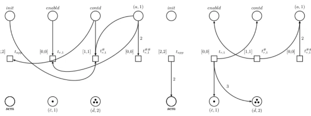
Fig. 4.The rule application phase for the Petri net, wherea∈w1andr=a→c(d, in2)3 andpromr(a) = 1,inhibr(a) = 2.
Next, we turn our attention to membrane systems with dissolution. LetΠ = (O, µ, w1, . . . , wn, R1, . . . , Rn, δ) be a membrane system with dissolution. We recall form our previous definitions that this means that there exists a special element δ ∈ O, which can appear on the right side of a rule only. Assume r ∈ Ri and δ∈rhs(r). Supposeris chosen in the actual maximal parallel rule application of mi. Then all the rules ofRi appearing in that computational step are executed as
usual, and, after the maximal parallel step is over, the regionmi disappears, its objects wander into the parent region and the rulesRicease to operate. With this in mind, we construct a time Petri net simulating the operation of the membrane system in the sense below.
Theorem 3.Let Π = (O, µ, w1, . . . , wn, R1, . . . , Rn, δ) be a membrane system with dissolution.
Then there is a time Petri netN= (P, T, F, V, m0, I)such thatN halts if and only ifΠ halts, and if they halt, then both systems provide the same result.
Proof. LetΠbe as in the theorem. We construct the Petri netNwith the required properties. The construction again leans on the proof of Theorem 1. The rule application phase is exactly the same with one exception: places δi symbolizing the dissolution of membrane mi appear. The difference manifests itself in the definition of the communication phase. Moreover, we introduce one more phase, a δ-phase, that serves for moving the elements of a previously dissolved membrane to the parent region. First of all, we define the set of places as before.
• P = P0∪P¯0∪ {initapp, initcom, sem, enabld, δi}, where P0 = O× {1, . . . , n}
and ¯P0 = ¯O× {1, . . . , n} and 1 ≤ i≤ n. Let m0(p) = wj(a) for every place p= (a, j)∈P0.
The only change is the presence of the places δi for every regionmi. Intuitively, they are indicators whether a membrane is going to disappear in the next step or has been dissolved already. This is reflected in the design of the arcs for the rule application phase. We require an extended set of transitions, since we have a third phase also that transfers the objects of the dissolved membranes to their parent membranes.
• T =T0∪T0∗∪T0δ∪T#∪T[∪ {tapp, tcom, tclean, t1sem, t2sem, t3sem},
and the arcs for the rule application phase are identical to those of Theorem 1 with the only exception of the arcs pointing fromti,j, whereri,j∈Ri, to the place δi with multiplicity 1 providedδ ∈rhs(ri,j). Thus we are only interested in the transitionsT0∗,T[and their corresponding arcs.
- LetT0∗={sa,i|a∈O, 1≤i≤n}andT0δ ={sδa,i |a∈O, 1≤i≤n}. Letmi
be a region other than the skin membrane, assumemkis its parent region. (Ifmi
is the skin membrane, it cannot disappear.) Let ¯p= (¯a, i)∈P¯0, then ¯p∈•sa,i
and, ifp= (a, i), thenp∈s•a,i. Moreover,initcom∈•sa,i∩s•a,i. In addition,δi
is connected withsδa,i for every objecta∈O, that is:δi∈•sδa,k∩sδa,i• and we have ¯q= (¯a, k)∈sδa,i•. Regarding the multiplicities, each arc has multiplicity 1.
Furthermore,I(sa,i) = [1,1],I(sδa,i) = [0,0] andI(tcom) = [2,2], wheretcom is the transition connectinginitcom with the placesem.
Intuitively, ifmi is a region with parent regionmk, the communication phase transfers the tokens of ¯p= (¯a, i) to the placep= (a, i), as long as the membrane
mi exists. When mi is marked for dissolution or has been already dissolved, that is, |δi| = 1, then the tokens of ¯p = (¯a, i) are redirected to ¯q = (¯a, k). This is achieved by a time gap between the possible firings of the transitionssa,iandsδa,i. This implies that the elements appearing on the right hand side of the rules of a dissolved membrane find their correct place: they wander to the upper levels of the tree until they find the first ancestor region not dissolved. The main ingredients of the construction are illustrated in Figure 5.
The only missing part is the subnet directing the remaining object of a dissolved membrane into an existing container membrane. We term this phase the cleaning phase. The construction is quite simple: letmk be a region and assume thatmi is its parent region. Then, for every place p= (a, k), there corresponds a transition tfplat which transfers the objects ofpto q= (a, i) whenδk contains a token. The placeinitclean is connected to all the transitionst[p in order to perceive when the tidying phase is ready. After this, 3 tokens are sent to the semaphore and a new application phase activates. More formally,
- letT[ ={t[a,k |a∈O, 1≤k≤n}. Assumemi is the parent region of region mk. Then p= (a, k)∈•t[p andq = (a, i)∈t[p• and δk ∈•t[p∩t[p•. Moreover, initclean ∈•t[p∩t[p• and initclean ∈ •tclean and sem ∈ t•clean. Regarding the multiplicities, each arc has multiplicity 1, except for (tclean, sem), which has multiplicity 3.
Furthermore,I(t[a,i) = [0,0],I(tclean) = [1,1].
This is described in Figure 6. The semaphore is extended with a new transition, t3sem which leads to the initialization of the third phase in the simulation of a maximal parallel step. The new semaphore is depicted in Figure 7.
Finally, we tackle the problem of the representation of membrane systems with priorities in terms of Petri nets. Again, our construction is a slight modification of the core model. We introduce some pieces of information in the simulation of the rule application phase that accounts for the treatment of the priorities. Let Π = (O, µ, w1, . . . , wn, R1, . . . , Rn, ρ) be a membrane system with priorities. This means thatρ⊆R×R, and the rule application is modified in the following way.
Definition 3.Let Π = (O, µ, w1, . . . , wn, R1, . . . , Rn, ρ) be a membrane system with priorities. Let r∈Ri, if1≤i≤n. Thenr is strong-applicable, if
1.ris applicable, that is, lhs(ri)≤wi, and
2. for everyr0 ∈Ri such that r0> r,r0 is not applicable.
Let r1, r2 ∈ Rk be two rules of region mk, assume that (r1, r2) ∈ ρ, that is, r1 > r2. Then, considering a computational step, r2 can be applied if r2 is applicable in the usual sense and, in addition, r1 fails to be applicable in the maximal parallel step belonging to region mk. We remark that we use priority in the strong sense: assume wk = a2b, r1 = a → c and r2 = ab → d. Then the result of the maximal parallel step will be ad, instead of cd, since r1 > r2 and
δ2 (a,2) (b,2)
tr
(¯c,2) ( ¯d,3)
2
(¯c,1) (c,2)
sδc,2
[0,0] [1,1] sc,2
(¯c,2) δ2
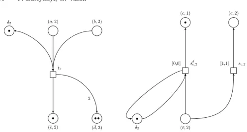
Fig. 5.The Petri net simulating a membrane system with dissolution. In this case,m2
is dissolved, hencesδc,2 can be activated moving the elements of ¯p(c,2) to ¯p(c,1).
sem (a,2) (a,1)
tclean
[1,1]
3
t[a,2 [0,0]
initclean
δ2
Fig. 6. The Petri net simulating the phase when the objects of a dissolved membrane are directed towards the parent membrane. Here we assume that region 1 is the parent of region 2, and the placeδ2 already has a token.
r1 is applicable, which implies thatr2 cannot be applied in that maximal parallel step at all, even ifr1is not applicable any more. The construction is again based on the basic construction, the only difference is that we have to pick out the applicable rules in order to obtain strong applicability. We do this by stratifying the various tasks due in the rule application phase with respect to time. Finding the strongly applicable rules takes place before the actual rule applications are simulated. Below, the placepAt
i will represent the strong applicability of ruleri.
sem
[2,2]
t1sem
[1,1]
t2sem
[0,0]
t3sem
initapp initcom initclean
1 2 3
Fig. 7.The semaphore for the Petri net with dissolution. The choice of the next phase is uniquely determined by the number of tokens arriving in the placesem.
Now we are in a position to state the theorem on the simulation.
Theorem 4.Let Π = (O, µ, w1, . . . , wn, R1, . . . , Rn, ρ) be a membrane system with priorities.
Then there is a time Petri netN= (P, T, F, V, m0, I)such thatN halts if and only ifΠ halts, and if they halt, then they provide the same result.
Proof. LetΠ as above. We describe the Petri netN simulatingΠ. The only dif- ferences in comparison with the model in Theorem 1 occur by the rule application phase when we select the transitions that are candidates for the strongly applicable rules. We omit repeating the communication phase and the alternating construc- tion of the Petri net in detail and we confine ourselves to the rule application phase only. The places are
• P=P0∪P¯0∪PA∪PB∪Pρ∪Pρ∗∪ {initapp, initcom, sem, enabld}, whereP0= O× {1, . . . , n}and ¯P0= ¯O× {1, . . . , n}and the auxiliary places are defined as in Theorem 1. Regarding the new places,PA={pAi,j |ri,j ∈Ri,1≤j ≤ |Ri|}
and P TB = {pBi,j | ri,j ∈ Ri,1 ≤ j ≤ |Ri|}. Moreover, Pρ = {pri>rj | p ∈ P0 and (ri, rj)∈ρ}, and Pρ∗={p∗ri>rj |p∈P0 and (ri, rj)∈ρ}.
The new places accomplish some bookkeeping in order to keep track of which rules are applicable and which ones are not. A token inpAi,j should symbolize the applicability of an arbitraryri,j∈Ri, while a token inpBi,j says thatri,jis blocked by an applicable rule of higher priority. The placesPρandPρ∗ensure that each pair ri,rj with (ri, rj)∈ρshould be checked only once with the purpose of dropping out the blocked rules. We define now the new transitions together with the arcs induced by these transitions.
• T =T0∪T0∗∪T#∪Tρ∪Tρ∗∪TN A∪T[∪ {tapp, tcom, t1sem, t2sem}.
The transitions are defined as before, except for the arcs in connection with the new sets of transitions. Regarding Tρ, where Tρ ={tri>rj | ri, rj ∈mk, (r1, r2)∈ ρ}
and T[ = {t[i,j | ti,j ∈ T0}. The arcs in connection with transitions T0, T0∗ and
T#, including the auxiliary transitions, are the same as in the core model. The differences emerge by the subnet checking strong applicability: if a rule r∈Ri is applicable, then a token is passed over topAt, wheretcorresponds tor. Moreover, when r0 ∈ Ri is applicable as well, and (r0, r) ∈ ρ, then the token in pr0>r is consumed and a token is transferred top∗r0>rand topBt. The token inpBt symbolizes thatris blocked in that maximal parallel step, which is expressed at time 1, when the tokens in pAt and pBt are both consumed by the transition tN A. When only tokens atpAt00 are left, where the corresponding ruler00is strongly applicable, then the usual rule applications take place with the refinement that transitions in T0
have places frompAas incoming places as well. After finishing with the simulation of the rule applications, the tokens remaining in PA are discarded, moreover, tokens are returned to Pρ at time instance 3.
- Let ri,j ∈ Ri, where 1 ≤ j ≤ |Ri|, 1 ≤ i ≤ n; then, as in the previous constructions,t#i,j∈T#is checking the applicability ofri,j. Letp= (a, i)∈P0
and let t#i,j ∈ T#; then p ∈ •(t#i,j)∩(t#i,j)• and initapp ∈ •t#i,j and enabld ∈
•t#i,j∩(t#i,j)•, which is a slight modification compared to Theorem 1. Enabled iw wired to eacht#i,j with both an incoming and an outgoing arc so that the process of finding the transitions for the strongly applicable rules can continue without hindrance. Furthermore,pAi,j∈(t#i,j)•.
Regarding the multiplicities, V((initapp, t#i,j)) = 1, and if f = (t#i,j, enabld) then V(f) = 1; furthermore, if f = (p, t#i,j) or f = (t#i,j, p) where p = (a, i), thenV(f) =lhs(ri,j)(a). in addition, the multiplicity of (t#i,j, pAi,j) is 1.
- Now, we turn to the operations of the transitionsTρ. Letri,j, ri,k ∈Ri with ri,k > ri,j. Then tri,k>ri,j ∈ Tρ, and for pAi,k and pAi,j, both of them are in
•tri,k>ri,j∩t•r
i,k>ri,j. Moreover,pri,k>ri,j ∈•tri,k>ri,j andp∗r
i,k>ri,j ∈t•r
i,k>ri,j. Furthermore,pBri,j∈t•r
i,k>ri,j and, ifrip∈Ri is arbitrary,pAtp andpBtp∈•tN Ap . Finally,∪Tρ∗ return the elements ofp∗r
i,k>ri,j back topri,k>ri,j, when the rule application phase is over. That’s why p∗ri,k>ri,j ∈ •t∗ri,k>ri,j and pri,k>ri,j ∈ (t∗r
i,k>ri,j)•.
The multiplicities of all the new arcs is 1.
The elements of T[ collect the tokens that might remain in the places PA when the simulation of the maximal parallel step is over. We havepAi,j ∈•t[i,j for every index pairi, j such thatt[i,j∈T[. The multiplicities of the arc is 1.
The elements ofT0 are extended with one more arc: for everyt ∈T0 we have pAt ∈•t∩t• with multiplicity 1.
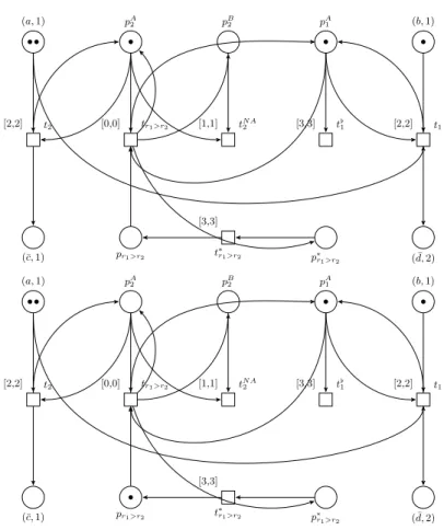
The timing makes sure that finding the strongly applicable elements precedes the rule applications themselves. For eachtri,k>ri,j ∈Tρ, we haveI(tri,k>ri,j) = [0,0], moreover, I(tN A) = [1,1] andI(t) = [2,2], if t ∈T0. Finally, I(t[i,j) = I(t∗r0>r) = [3,3].
- Regarding ti,j ∈ T0, where 1 ≤ i ≤ n and 1 ≤ j ≤ |Ri| is as before, let p= (a, i) ∈•ti,j if and only if a∈lhs(ri,j). In addition, enabld∈•ti,j∩t•i,j (1≤i≤n,1≤j≤ |Ri|).
(a,1) pA2 pB2 pA1 (b,1)
t2
[2,2] [0,0] tr1>r2 [1,1] tN A2 [3,3] t[1 [2,2] t1
(¯c,1) pr1>r2 p∗r1>r2 ( ¯d,2)
[3,3]
t∗r1>r2
(a,1) pA2 pB2 pA1 (b,1)
t2
[2,2] [0,0] tr1>r2 [1,1] tN A2 [3,3] t[1 [2,2] t1
(¯c,1) pr1>r2 p∗r1>r2 ( ¯d,2)
[3,3]
t∗r1>r2
Fig. 8. Assumew1 =a2bandr1,r2∈R1,r1 =ab→d,r2=a→csuch thatr1> r2. Then onlyt1can fire: transitiontr1>r2 delivers a token to placepB2, and at time instance 1 the tokens frompA2 andpB2 are removed by transitiontN A2 .
As regards the weights of the arcs, letp= (a, i) andf = (p, ti,j)∈F. Then the weight off is the multiplicity of a∈ O on the left-hand side of ri,j, namely, V(f) = lhs(ri,j)(a). If f = (ti,j, enabld) orf = (enabld, ti,j), thenV(f) = 1 (1≤i≤n,1≤j≤ |Ri|). Moreover, iftapp is the transition connectingenabld tosem, thenI(tapp) = [4,4].
The definition of the communication part is the same as that of the proof of Theorem 1, we ignore omit repeating the construction. The main changes compared
to the core model can be seen in Figure 8.