325 1

D A M P I N G A N I N E R T I A L N A V I G A T I O N S Y S T E M Charles B r o x m e y e r *

Massachusetts Institute of Technology, C a m b r i d g e , M a s s . A B S T R A C T

W h e n an inertial navigation system designed for a freely m a n e u v e r a b l e vehicle is excited by the r a n d o m drift of its gyros, error oscillations develop which tend to build up with time. T h e system equations can be modified so that the root- m e a n - s q u a r e values of the errors approach limiting values;

however, such a modification invariably introduces an unde- sired response of the s y s t e m to vehicle motion. It can be s h o w n that the p e r f o r m a n c e of an inertial navigation system m a y be expressed so that the responses of the vertical errors, and of the azimuth error, to gyro drift display a strong anal- ogy to the closed loop response function of a simple servo- m e c h a n i s m . B y pursuing this analogy, using standard tech- niques of s e r v o m e c h a n i s m theory, the ultimate p e r f o r m a n c e limitations on the d a m p e d inertial navigation system can be displayed and specific d a m p i n g equalizers designed.

I N T R O D U C T I O N

T h e errors of an inertial navigation system arise f r o m the various c o m p o n e n t imperfections, f r o m the theoretical approximations that have been built into the system, and f r o m inaccuracies in the setting of initial conditions. T h e m o s t serious source of navigation s y s t e m errors is gyro drift.

Analysis s h o w s that constant gyro drift, or an impulse of gyro drift, will cause sustained oscillations. T o the accu-

Presented at A R S Guidance, Control, and Navigation Conference, Stanford, Calif., A u g . 7-9, 1961.

1 Staff M e m b e r , Instrumentation Laboratory.

racy that constant or other predictable gyro drift can be m e a - sured, it can effectively be compensated. T h e r e r e m a i n s a r a n d o m , in general n o n c o m p e n s a b l e , c o m p o n e n t of gyro drift that will act on the system like a succession of small i m - pulses. T h e effect of the r a n d o m drift is cumulative, and the

resulting error oscillations will tend to g r o w with time. It can be s h o w n that the r o o t - m e a n - s q u a r e ( r m s ) value of the error oscillations increases as the square root of time.

If a single impulse of gyro drift produced a d a m p e d error response instead of producing a sustained sinusoidal response, the effect of a train of impulses would not tend to accumulate, since the effect of each m e m b e r of the train would disappear with time. It is seen, therefore, that f r o m the standpoint of the effect of gyro drift on a system, it would be highly de- sirable that the response to a single impulse be a d a m p e d function; this situation that would be realized if the poles of the system response functions had negative real parts instead of being pure imaginary quantities.

Therefore, the possibility might be considered of m o d i - fying the navigation system equations so that the poles of the

system response functions all acquire negative real parts. It will develop that such a modification is possible. In this paper, the m e t h o d s by which the modified set of system equa- tions can be obtained, and the advantages and disadvantages of using such a set of equations, will be explored.

It is immediately apparent that if the design of an inertial navigation system is modified in any respect that requires a change in the ideal specific force equations, the system will develop errors that depend on vehicle acceleration. F o r an aircraft, the effect of the high accelerations that m a y occur could be so severe that a d a m p e d s y s t e m would not be useful.

F o r slow speed vehicles, h o w e v e r , the errors introduced in a d a m p e d system by changes of motion are small, and it is profitable to consider the creation of a favorable balance be- tween such errors and the reduction in the errors excited by r a n d o m gyro drift.

If externally derived velocity information is available, a compensating modification is possible. It is k n o w n that

velocity information, properly injected into a d a m p e d inertial

navigation system, can return the s y s t e m to a state in w h i c h errors are not excited by vehicle accelerations and in w h i c h the desired d a m p i n g effect on gyro drift-excited errors is

still achieved. A serious objection to such a procedure is that the accuracy of the external velocity information m u s t rival that p r o d u c e d by the navigation s y s t e m itself. T h e r e is, therefore, implied as an element in such a hybrid system, a completely redundant s y s t e m w h o s e only function is to provide compensation for the d y n a m i c effects of damping. U s e of such a s y s t e m m a y be considered questionable. In the follow- ing discussion, h o w e v e r , the m e t h o d of introducing externally m e a s u r e d velocity into an inertial navigation s y s t e m will be considered.

T H E E F F E C T O F A R A N D O M I N P U T O N A L I N E A R O S C I L - L A T O R

T h e case of a linear oscillator excited by a r a n d o m input function is considered first. This e x a m p l e will prove directly applicable to the navigation s y s t e m p r o b l e m .

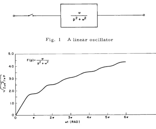
T h e s y s t e m to be e x a m i n e d has one input and one output and can be represented as a transfer function as s h o w n in Fig. 1. It is supposed that the switch s h o w n in Fig. 1 is closed at time t = 0, and that the input to the s y s t e m is a ran- d o m function having a zero m e a n and a constant r m s value.

T h e output of the s y s t e m will be an oscillatory r a n d o m func- tion, and the peak amplitudes will tend to g r o w with time.

Since the output is zero, up to the instant the switch is closed, and g r o w s with time thereafter, it is not a m e m b e r of a sta- tionary r a n d o m process and it is not possible to determine an r m s value by averaging with respect to time. A n r m s value can be defined, h o w e v e r , by considering an e n s e m b l e of linear oscillators, all energized at t = 0 by stationary ran- d o m input functions having the s a m e statistics. T h e r m s value is defined by taking an average over the entire e n s e m b l e at a given time.

Using the properties of the input process, and of the os- cillator, it is possible to calculate the r m s value of the out- put process, as a function of time, by using the equation

e2(t) = f Γ φ(χ - y)£(t - x)f(t - y) d x d y [ l]

w h e r e e^(t) is the m e a n - s q u a r e error, φ(τ) is the autocorrela- tion function of the input process, and f (t) is the response of the system to a unit impulse (1). ^ Eq. 1 holds for general s y s t e m s and is not limited to the oscillator under discussion.

F o r the linear oscillator s h o w n in Fig. 1, the response to a unit impulse function is simply

f(t) = sin cot [2]

Valid use of Eq. 1 to predict an average error n o w re- quires that the function φ(τ) be the autocorrelation function of gyro drift and that it be suitably obtained f r o m experimental data. F o r the i m m e d i a t e purpose of the discussion, which is to observe the general effect of d a m p i n g on the r m s errors, and to c o m p a r e the effectiveness of various d a m p i n g m o d e s , it will be a s s u m e d that the s y s t e m input is white noise. This is equivalent to a s s u m i n g that the input process has a flat average s p e c t r u m over the system pass band. T h e a s s u m p - tion introduces an analytical simplification, and will not affect the design of the equalizers to be developed later in the paper, since they are not designed with an explicit dependence on the statistics of gyro noise.

T h u s

φ(τ) - π Ρ δ ( τ ) [ 3]

the autocorrelation function of white noise. T h e function δ (τ) is the unit impulse function, and Ρ is the average p o w e r per unit bandwidth. T h e autocorrelation function is the Fourier transform of the p o w e r spectral density, and the factor π in Eq. 3 arises f r o m the convention e m p l o y e d in writing the Fourier integral t h e o r e m as a set of direct and inverse trans- f o r m s .

l u m b e r s in parentheses indicate References at end of paper.

e2(t) - π Ρ

Γ Γ

J0 ^Jo

f2(t - y) dy [4]

0

Substituting Eq. 2 in Eq. 4, the r m s value is obtained as

e (t) = ~z (cot + — sin 2 cot) ^L

/ Ζω 2ω A plot of the function

cot + (ΐ/2ω) sin 2 cot

is s h o w n in Fig. 2. It is apparent f r o m Eq. 5 and f r o m the figure that increases as the square root of time.

T h e r m s output of a d a m p e d linear oscillator having a transfer function

F(p) =

— 2 [6]

ρ + 2 ζ ρ ω + ω

is n o w considered. T h e impulse response is the d a m p e d function

η Χ ω -at . P_ η

f(t) = — e sin ßt [7]

w h e r e

a = ζ ω and

With Eq. 3, the m e a n - s q u a r e value of the output b e c o m e s

β - ω / 1 - ζ2

2

If J e (t) is calculated for the d a m p e d system, as before, it is found that a steady value is approached. If

α/β = η then the m e a n - s q u a r e value is

e2(t) =

4 ω / 1 - ζ2

1 - e

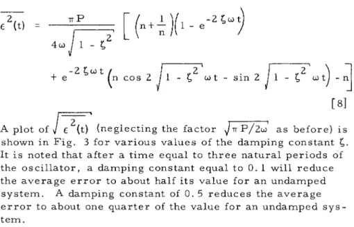
+ e (η cos 2 / 1 - ζ w t - sin 2 / 1 - ζ α [8]

A plot of J €^(t) (neglecting the factor ^ π Ρ/2ω' as before) is s h o w n in Fig. 3 for various values of the d a m p i n g constant ζ.

It is noted that after a time equal to three natural periods of the oscillator, a d a m p i n g constant equal to 0. 1 will reduce the average error to about half its value for an u n d a m p e d system. A d a m p i n g constant of 0. 5 reduces the average error to about one quarter of the value for an u n d a m p e d sys- tem.

Fig. 4 s h o w s a similar set of average errors for the sys- t e m w h o s e transfer function is

F ( p ) =

—

ρ + 2 ζ ω ρ + ω

T h e general behavior of the curves is similar to that obtained for the system of Fig. 1, and the final values are the s a m e for the s a m e values of the d a m p i n g constant.

S I M P L I F I E D I N E R T I A L N A V I G A T I O N S Y S T E M

A highly simplified m o d e l of an inertial navigation sys- t e m is n o w considered. T h e system is a s s u m e d to be con-

strained to m o v e only over a meridian. It has a single axis, n o r m a l to the plane of the meridian, and is designed to indi- cate the vertical and c o m p u t e latitude. T h e case of a three- axis s y s t e m will be treated in a later section; it should be noted that the behavior of the single-axis system described here is the s a m e as the behavior of a three-axis system about its north pointing axis w h e n the navigation s y s t e m is located at the equator.

A block d i a g r a m of the s y s t e m showing the signal flow and the effect of an error in vertical indication as a feedback sig- nal affecting the accelerometer output is s h o w n in Fig. 5.

T h e establishment of the block d i a g r a m of Fig. 5 is treated in Ref. Ζ (pp. 9-12). It is noted that the figure contains a block representing an as yet undetermined transfer function H(p).

Writing the vertical error β as a function of the north velocity ω and the gyro drift U, the result is

g / R

s/R

g / R

ι +

ι +

&φ

Ρ2 ρ2

F o r an unmodified s y s t e m the transfer function H(p) is equal to 1. In this case the first t e r m on the right-hand side of the equation disappears, and the error angle β b e c o m e s

β = u — £ [11]

Ρ + g / R

which is analogous to the case of the linear oscillator con- sidered in the previous section.

B y suitably selecting the function H , the response of the system to gyro drift can be d a m p e d . If Η is different f r o m 1, h o w e v e r , the nonvanishing factor 1 - Η in the first t e r m s h o w s that vehicle motion will contribute a c o m p o n e n t to the error p.

It is desired to m a k e the function

2

Ρ

be equivalent to the response function of a d a m p e d oscillator.

If this function is written in the f o r m

1 Ρ²

Ρ

it is apparent, since the second factor has the appearance of a single loop s e r v o m e c h a n i s m response function

Y/(l + Y)

that conventional s e r v o m e c h a n i s m synthesis techniques m a y be e m p l o y e d to develop an equalizer transfer function H. T h e function

G =

U 2

Ρ

m a y be conveniently represented graphically by m a k i n g the substitution

ρ = ι ω expressing the result in the f o r m

G(ico) = 1 G (ω) I βί θ (ω)

and then plotting the gain function

M = 20 log 1 G (ω) | and the phase shift function

θ = θ (ω)

against the logarithm of ω (see Ref. 3 or any text on servo- m e c h a n i s m theory).

T h e gain of G(ioo) will be plotted as a line having a slope of 12 db per octave, crossing the zero db line at the angular frequency

T h e phase shift will be a constant negative angle of 180° over the entire frequency range.

E l e m e n t a r y s e r v o m e c h a n i s m theory indicates that this is a situation in which the system is at the boundary of stable behavior, and that a disturbance will cause the system to have sustained oscillations.

T h e response can be i m p r o v e d by selecting the design of the cascaded equalizer Η so that the gain of the function

crosses the zero db line before a condition of 180° phase shift is reached.

It is apparent that the function Η need be different f r o m 1 only in the neighborhood of the frequency J g/R.' T h e de- sirability of maintaining the t e r m 1 - Η as small as possible s h o w s that the function Η should be different f r o m 1 over as n a r r o w a frequency band as possible.

It is supposed that Η is required to be a lead function ω s

Η ( ί ω ) G(ico)

+ ω

ο ω < ω

ο [12]

ω ρ + ω 1

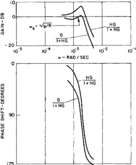
having a value of one at low frequencies. Eig. 6 illustrates:

1) the undamped navigation system response curves; 2) the frequency response of H for an appropriate selection of the constants CA )

and ω-μ and 3) the frequency response of the combination H G .

The phase shift curve is - 180° at low frequencies and then becomes less than 180° in magnitude in the region where the gain curve crosses the zero db axis. According to funda- mental servomechanism theory, the resulting closed loop

system should be stable.

Fig. 7 shows the response function plotted as a curve on a gain vs. phase shift diagram. A diagram of this type is sometimes called a Nichols chart. The contour lines of the chart are lines of constant gain and phase of the closed loop response function. It is apparent from the figure that the modification provided by the function Η allows the character- istic to bypass the critical (0 db, - 180°) point on the gain- phase diagram.

The closed loop response curves representing the func- tions

HG/(1 + H G ) and

G/(l + H G )

are shown in Fig. 8. The resultant closed loop response function has been adjusted to peak at 1 db.

Another possible equalizer transfer function Η can be realized by simply bypassing the first integrator of the navi- gation system with a direct connection. For this case, the transfer function can be written

Η = 2 ζ jR/g' ρ + 1 [13]

Fig. 9 shows the gain and phase shift characteristics of this

function. The necessary positive phase shift is obtained but

unnecessary gain and positive phase shift is continued into the

high frequency region. A s might be suspected, this condition produces an undesired response to sudden vehicle motions.

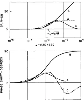
Fig. 10 shows the gain and phase shift characteristics of several equalizer transfer functions. The functions corres- ponding to curves A and Β have already been considered. The transfer function illustrated by curve C has a gain of zero db at high frequencies and at low frequencies and, according to the criterion that 1 - Η should be as small as possible, would be expected to contribute less error because of vehicle m o - tion.

Fig. 11 shows the result of a one-knot step in vehicle velocity on the vertical error for all three cases. The closed loop response function w a s adjusted to peak at 1 db in each case.

A s mentioned, the function Η that introduces excessive gain and phase shift at high frequencies has a response that is inferior to that resulting from use of the other two func- tions. Between the two functions shown in curves A and C of Fig. 10, there seems little choice. It m a y be concluded that the small gain contributed by the Η function first considered has negligible effect because of the attenuation of the closed loop system transfer function that multiplies (1 - H) in Eq. 10.

T H E A Z I M U T H E R R O R

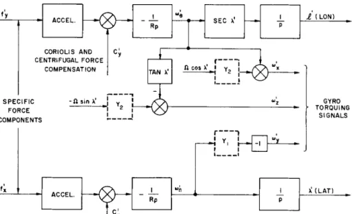
To determine the behavior of the azimuth error of a damped inertial navigation system, it is assumed that the navigation system to be considered is the one illustrated in Fig. 12. This is a very general system whose behavior, in the undamped case, is discussed in Ref. 2 and 4. In the un- damped case, the blocks shown dotted are not included. For the present, the blocks represent unknown transfer functions which, it is hoped, will produce the desired damped behavior of the system. To avoid introducing unnecessary complexity in this description, the equations will be developed for the simplified case of a system in a vehicle near the equator.

The corresponding equations for a vehicle at any latitude can be developed by a similar but m o r e detailed analysis. For

simplicity, the 84-min oscillations will be considered un-

damped, and concern will be with only the m o r e important

24 hr oscillations.

It can readily be shown that vertical errors about north and east, α and β, satisfy the following two equations

δ ώ = (g/R) β

[14]

δ ώ = - (g/R) α

w h e r e δ ω and δ ω are the errors in north and east angular n e

velocity computation. Also, if ω , ω , and ω are the angu- lar r a t e components of a geograpnic C o o r d i n a t e system w i t h origin at the vehicle, and if ω' , ω' andco' are the corres- ponding computed rates that are used to torque the three

gyros, then the vertical errors and the azimuth error γ satisfy

α = ω' - ω - γω + βω + U χ χ y ζ χ

β = ω' - ω - α ω + γ ω + U Γ15]

y y ζ χ y

γ = ω' - ω - β ω + α ω + U

ζ ζ χ y ζ

w h e r e U , U , and U are the drift rates of the x, y, and ζ x y ζ

gyros.

The last equation of this set is considered. F o r general vehicle motion, the term ω ^ is given by

ω = - Ω sin λ - ω tan λ Γ16]

ζ e w h e r e λ is the latitude.

The torquing signal ω¹ would, in the u n d a m p e d case, be

ω" - - Ω sin λ¹ - ω' tan λ' [17]

ζ e ^L

In the d a m p e d case, this expression is modified and the ζ gyro is torqued with a term

ω' = - Υ (Ω sin λ¹) - ω' tan λ' [ 18]

ζ

Ζ

T h e function Υ ^ corresponds to one of the blocks indicated in Fig. 12. It should be noted that the second t e r m of this ex- pression is not modified. A positive or negative ωβ will

change the resonant angular frequency of the system f r o m the v a l u e d to s o m e neighboring value, but it is a s s u m e d that the vehicle is slowly m o v i n g and that the resonant angular fre- quency is effectively dependent only on the first term.

If the differences are f o r m e d between c o m p u t e d and actual rates around z, and the c o m p u t e d angle λ¹ is replaced by (λ + δ λ) and the c o m p u t e d rate by (coe + δ ωβ) , then

ω' . ω = » γ Ω cos λ δ λ + (1 - Y ) Ω sin λ

ζ ζ 2

Ζ

- ω β β ο ^ λ δ λ - δ ω tan λ Γ19]

e e N e a r the equator, the entire expression for y b e c o m e s

y = . γ Ω δ λ - δ ω λ - β Ω - α ω + U

1 Ζ e Μ η ζ

+ (1 - Υ2) Ω λ [ΖΟ]

T h e t e r m s δ ωΘ λ and α,ωη m a y be neglected in c o m p a r i s o n with the other t e r m s , and the resulting equation is

y = - Υ Ω δ λ - β Ω + ( 1 - Υ ) Ω λ + υ [Zl]

c, ù Ζ

If a similar procedure is applied to the β equation, another equation of the s a m e type m a y be developed. The three equa- tions

δ ώη = "f ß

ß = - Υ^χ δ ωη + Ω Ύ + Uy + (1 - Χ \ ωη [22]

y = - Υ Ω δ λ - β Ω + U + ( 1 - Υ ) Ω λ

and the definition

δλ = δ ω

[23]

are seen to describe the behavior of the variables δ ω

, λ, β, and 7 , and the equations for δ U>

and α m a y be handled inde- pendently.

If this set of equations is solved for

in terms of the vehicle velocity ω

, and the gyro drift rates ΙΙ

, U and U

one obtains

Ύ =

3 2 Ρ

L 1 + Y

Ω 3 2

Ρ

Ω υ +

2 Υ

1 + Υ

3 —

Ρ

Ω

+ - - r (— ρ² + 1)(1 - Υ³) Ω ω^η 1 + Υ Ω² g

3 2

[24]

where

(R/g)

/

3 (R/g) ρ2 + YL

[25]

Eq. 24 is directly analogous to the equation that w a s used to

describe the vertical error in the single-axis case considered

previously. Each disturbing influence is modified by a trans-

fer function that is in the form of a closed loop response

function, and can obviously be handled by the servo tech-

niques that were applied earlier. The presence m a y be noted

of the factor 1 - Y 3 in the last term, which shows that when

is equal to

, no error will result from vehicle motion.

W h e n a satisfactory f o r m has been found for Y ^ , it is necessary to break it up into c o m p o n e n t s Y^ and Y 2 which are m e c h a n i z e d individually by the navigation system. T h e selection of Y^ and Y 2 has been m a d e on an arbitrary basis by letting Y± equal 1 and solving for Y 2 . Since the w a y that Y 3 is broken up will not affect 7 , the criterion to be used is the magnitude of the effect on the vertical errors. It can be s h o w n that the arbitrary selection of Y ^ as 1 will give satis- factory results.

T h e synthesis procedure for Y ^ is similar to the one used to find the H function. Rather than repeat the discussion of the synthesis procedure, s o m e of the results will be given for various values of an effective d a m p i n g constant ζ. Experi- mentation s h o w s that the shape of the characteristic Y 3 has little effect in changing the response to motion provided that the s a m e effective d a m p i n g constant is used and the closed loop response functions

Y³ ( Ω²/^{Ρ 2})

1 + Y 3 ( Ω2/ Ρ2) and

(Ω²/ρ²) 1 + Y s ( Ω²/ ρ²)

have unity gain at low frequencies. A n effective value of ζ corresponds to peak values of the gains of the two closed loop response functions. F o r example, ζ = 0. 5 corresponds to a peak gain of 1 db for the second of the two functions listed.

T h e insensitivity of the s y s t e m to modification by a Y 3 that has a high gain at frequencies above Ω, s e e m s to result f r o m the presence of an integration in the last t e r m of Eq. 24 as c o m p a r e d with the last t e r m Eq. 10. This condition differs f r o m the situation that occurred in the case of vertical d a m p - ing, w h e r e it w a s apparent that s o m e advantage could be de- rived by careful shaping of the modifying transfer function.

If a vertical error equalizer function H is included Eq.

24 is unchanged. H o w e v e r Y3 b e c o m e s

(R/g) ρ + Y j Η

If Η is appropriately selected, it can be s h o w n that the re- sponse of the system to motion along a meridian differs little f r o m the case in w h i c h Η is neglected.

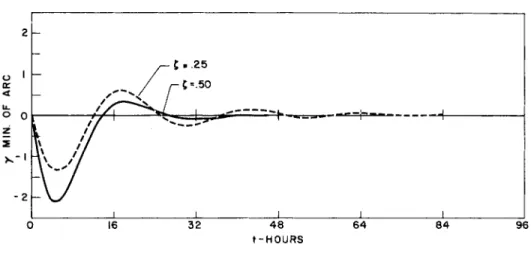
Figs. 13, 14, and 15 s h o w the response in azimuth error, under this assumption, for a step function input and various values of the d a m p i n g constant.

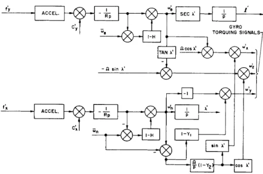
If external velocity information is available, it m a y be introduced as s h o w n in Fig. 16. If the external velocities ω^η and cö~^e are precisely measured, the connections shown will eliminate the component of error resulting from vehicle motion. Except for the external inputs and the vertical error equalizers H, the diagram can be shown to be equivalent to that of Fig. 12.

T h e operation of a d a m p e d five-gimbal system can be given in completely analogous form with that of the three- gimbal system that has been considered.

A n u n d a m p e d five-gimbal system can be arranged which does not require torquing of the system gyros. T h e input axes of the gyros define an orthogonal system which is ro- tated so that it always maintains almost the s a m e orientation with respect to the figure of the earth, but no gyro is rotated about its input axis. Torquing signals m u s t be provided for damping, however, and Fig. 17 shows the damping signal resolution for a system in which one gyro input axis is paral- lel to the polar axis, another input axis points east, and the third axis points toward the polar axis, and is parallel to the equatorial plane. T h e diagram is equivalent to that of Fig.

16.

R E F E R E N C E S

1 Laning, J. Η . , Jr. and Battin, R. Η . , R a n d o m P r o c e s s e s in Automatic Control ( M c G r a w - H i l l B o o k C o . , Inc., N e w Y o r k , 1956) C h a p . 6.

2 B r o x m e y e r , C . , "Analysis of an Inertial Navigation S y s t e m , " R e p . R - 2 4 1 , M . I . T . Instrumentation Laboratory, C a m b r i d g e , 1959.

3 B r o w n , G. S. and C a m p b e l l , D . P. , Principles of S e r v o m e c h a n i s m s (John Wiley and Sons, Inc. , N e w Y o r k ,

1948) C h a p . 8.

4 B r o x m e y e r , C . , "Foucault P e n d u l u m Effect in a Schuler-Tuned S y s t e m , " Journal of the A e r o / S p a c e Sciences, M a y , I960.

ο

ω

ρ 2 + ω2

Fig. 1 A linear oscillator

5 . 0

ω\

Fig. 2 R M S output of u n d a m p e d linear oscillator excited by white noise

3 i r 4w u/t (RAD)

Fig. 3 R M S outputs of d a m p e d linear oscillators excited by white noise

5 . 0

Fig. 4 R M S outputs of d a m p e d linear oscillators excited by white noise

- R P " n \ ¹

R P H(p) 1

) Ρ

1

R P H(p) 1

Ρ

•<3ß -ß

Fig. 5 Single loop system

2 0

- 2 0

(P)

/ H ( p )

/

ω8 =Vg7FT ^(p)H(p)

ω 2 7

ω Lü

ο: 0 ο

LU

180*

10" 10"^ 10"

ω - RAD/ SEC

__H(p)

G(p)H(p) 1 PHASE MARGIN 10'

6 Gain and phase shift v s0

log angular frequency (open loop)

G(p)H(p)

GAIN (CLOSED LOOP)

P H A S E L O S E D LOOP)

- 2 0

-180 - 1 4 0 - 1 0 0 - 6 0 P H A S E (OPEN LOOP)-DEG.

- 2 0

F i g o 7 Gain v s⁰

phase diagram

1 0 ,

FIGO 8 Gain and phase shift v s⁰

log angular frequency (closed loop)

2 0

ο

-

/

^ R / g ' p+l

χω5 = T I T R

1 0 "5 I 0 "4 I 0 "3 1 0 2 1 0 " '

« - R A D / S E C

FIGO 9 Gain and phase shift vs, log angular frequency of

simple lead equalizer

Figo 11 Verticle error for one knot step input

ACCEL.

- < g > -

CORIOLIS AND CENTRIFUGAL FORCE

COMPENSATION

Rp SEC λ' 1

Rp SEC λ'

Ρ

TAN λ' Λ cos λ' I γ„

Μ τ2

SPECIFIC FORCE COMPONENTS

- Λ sin λ' ! γ J

Ί Υ2 \~

• I

ACCEL. I

Rp

-Ι . "Li

Ζ (LON)

GYRO TORQUING

SIGNALS

λ' (LAT)

Figo 12 Damned three-axis inertial navigation system (three gimbal)

Fig. 13 A z i m u t h error for one knot step input

2 h

I ι ι ι ι ι

I

0 16 3 2 4 8 6 4 8 4 9 6 t - H O U R S

Fig. 14 A z i m u t h error for one knot step input

-

ζ = . 7 5 — \

j Λ — j j_ IM 1 1 1 1

ft / /

'

I 1

0 \\J/ 16 3 2 4 8 6 4 8 4 9 6

t - H O U R S

Fig. 15 A z i m u t h error for one knot step input

ACCEL.

ACCEL.

1 Rp

1

Rp \

/Γ

\

- f t sin λ

SEC λ' I

SEC λ'

Ρ GYRO TORQUING SIGNALS-i

TAN λ' ft cos λ'

I Rp

i - Y i

sin λ'

cos λ'

Figo 16 Damped three-axis inertial navigation system with

external velocity compensation

ACCEL. 1 _ι J

Rp _

Λ| LON DRIVE

SEC λ' ftt + i

ACCEL. 1

Rp ^\

-<SH

LAT DRIVE

l-Y, l-Y,

9- ( , - v2, 9- ( , - v2,

LAT (Y) GYRO

EQ (Z) GYRO

Fig

(five gimbal)