Control Strategies, Robustness Analysis, Digital Simulation and Practical Implementation for a Hybrid APF with a Resonant Ac-link
Yang Han
1, Lin Xu
2, Muhammad Mansoor Khan
2, Chen Chen
21Department of Power Electronics, School of Mechatronics Engineering, University of Electronic Science and Technology of China, No.2006 XiYuan Road, West Park of Chengdu Hi-Tech Zone, 611731 Chengdu, P. R. China
2Department of Electrical Engineering, XuHui Campus, Shanghai JiaoTong University, #1954 HuaShan Road, 200030 Shanghai, P. R. China
E-mail: hanyang_facts@hotmail.com, xulin198431@hotmail.com
Abstract: This paper proposes a novel hybrid active power filter (HAPF) topology based on the cascaded connection of the AC-side capacitor and the third-order LCL-filter, which has the advantage of the conventional hybrid filter and the LCL-filter in terms of reduced dc- link voltage and better switching ripple attenuation. The robust deadbeat control law is derived for the current loop, with special emphasis on robustness analysis. The stability and robustness analysis under parameter variations are presented for the converter-side current tracking scheme and the grid-side current tracking scheme. It is found that the stability margins obtained from the converter-side current tracking control scheme are generally higher than those obtained from the grid-side current tracking scheme. However, the converter-side current tracking scheme is sensitive to the variation of the damping resistance, and it would impose additional parameter uncertainty on the control system and complicate the problem. Hence the grid-side current tracking scheme is implemented. The simulation results obtained from Matlab/Simulink are presented for verification, where the inductance variation and grid disturbance scenarios are also taken into consideration. The effectiveness of the proposed hybrid APF is substantially confirmed by the simulation and experimental results.
Keywords: power quality; harmonic estimation; active filter; hybrid; robustness analysis;
digital signal processor (DSP)
1 Introduction
Due to the proliferation of nonlinear loads in electric power distribution systems, electrical power quality has been an important and growing problem Particularly, power quality problems are causing detrimental effects for customers; these problems result from current harmonics produced by nonlinear loads, e.g., variable ac motor drives, HVDC systems, arc furnaces, grid-connected renewable energy resources and household appliances. The increased harmonic pollution causes a significant increase in line losses, instability, and voltage distortion when the harmonic currents travel upstream and produce voltage drop across the line impedance [1-3]. This fact has led to the proposal of more stringent requirements regarding power quality, like those specifically collected in the standards IEC- 61000-3-{2,4} and IEEE-519 [4, 5]. For several decades, active power filters (APFs) have been recognized as the most effective solutions for harmonic compensation. Their objective is to suppress the current harmonics and to correct power factor (PF), especially in fast-fluctuating loads [2]. A lot of recent literature has tried to improve APFs by developing new topologies or new control laws [3, 6-8]. In order to provide a systematic elaboration of the recent development in APFs, a survey of the state-of-the-art techniques for the APFs is outlined herein.
It was reported in Refs. [9-13] that the performance of APF is dependent on how the reference compensating signals are generated. The instantaneous reactive power theory [9], the modified p-q theory [10], the synchronous reference frame (SRF) theory [11], the instantaneous id-iq theory [12], and the method for the estimation of current reference by maintaining the voltage of dc-link [13] are reported for generating references through the subtraction of positive sequence fundamental component from the nonlinear load current. These control schemes look very attractive for their simplicity and ease of implementation, but fail to provide an adequate solution under extreme conditions of harmonics, reactive power and their combinations, with limited power rating of voltage source inverter (VSI) [14]. In such cases, to safeguard the hardware, the protection scheme isolates the APF, which leaves the system to the mercy of unwanted disturbances;
or, if reference signals are saturated, then the APF becomes a source of disturbance itself. In [15], the reference generation method based on the Goertzel algorithm was proposed; however, some practical issues, i.e, the stability of the closed-loop current control algorithm and voltage regulation, have not been discussed. Other solutions to harmonic detection and reference signal generation are based on artificial intelligence (AI), particularly on neural networks (NNs) [16]. In recent literature, a slightly different approach was proposed in [17], where an adaptive linear neural network (ADALINE), trained by a least-squares algorithm (LS) [18], was used to estimate the active component of the fundamental load current. In [19], a single-phase distributed generation (DG) unit with APF capability via adaptive neural filtering (ANF) was introduced, and which does not need a priori training of the neural network. Hence it is neither
cumbersome nor computationally demanding, especially if compared with other neural-based techniques that require offline training [16].
Apart from the neural network approach, the genetic algorithm (GA) was also introduced for APF applications [20]. These control strategies have a common drawback concerning the global stability of the closed-loop system, which hampers its application for practical APF systems. To overcome the stability issues, the sliding-mode control (SMC) was presented in [21]. However, the calculation technique for the reference current using SMC scheme is complicated and would require more advanced and sophisticated hardware for the practical implementation of the algorithm. The direct power control (DPC), on the other hand, is an indirect current control method that originates from the instantaneous reactive power theory (IRPT) [22]. However, the main drawback of DPC is the high gain of the controller and, as a consequence, the values of the input inductors have to be very large to attenuate the current ripple, which increases the cost, size, and weight of the system [22, 23]. Recent works have introduced predictive control and model-based strategies for DPC with improved steady state and dynamic response [23], where the control loops is designed with a high gain at the selected harmonic frequencies. In [24], repetitive control was utilized for harmonic compensation, which achieves low total harmonic distortion current waveforms, but at the expense of fast sampling capabilities of the hardware. As an alternative approach, resonant harmonic compensators were presented in [25], which were based on generalized integrators connected in parallel with a conventional tracking regulator. Moreover, deadbeat current control schemes were reported in [26]; these offer the potential for achieving the fastest transient response, more precise current control, zero steady-state error, and full compatibility with digital control platforms. However, there are two main practical issues related to the deadbeat control, namely: 1) bandwidth limitation due to the inherent plant delay and 2) sensitivity to plant uncertainties.
In addition to the reference current generation schemes and the current control algorithms, the switching ripple attenuation and the electromagnetic interference (EMI) reduction are also of vital importance for the practical implementation of APFs. To resolve the issues of switching ripple and EMI reduction, normally a large value inductance for output filtering should be adopted [27]. However, a high value inductance degrades system dynamic response and also requires a higher voltage on the dc-link of the inverter, thus resulting in higher power losses.
By connecting a small-rated active filter directly to the single-tuned LC-filter to form the hybrid topology, the dc-link voltage of the VSI can be reduced to a fraction of the mains voltages. In [27], an alternative solution for switching frequency reduction using LCL-filter-based topology was presented.
In order to take the advantage of the hybrid LC-filter topology for reduced dc-link voltage and the LCL-filter for better switching ripple attenuation, a novel hybrid APF (HAPF) configuration is proposed in this paper. It resembles the single-tuned LC-filter-based hybrid topology at lower frequency range, and thus the dc-link
voltage of the VSI is remarkably reduced. By using a third-order LCL-filter to replace the L-section of the resonant LC-filter, the total filter inductors are significantly reduced and satisfactory switching ripple attenuation is achieved. The adaptive linear neural network [28] is utilized for harmonic estimation and reference current generation for the proposed hybrid APF. Additionally, the deadbeat control law [26] is derived based on the low frequency equivalent model of the LCL-filter section of the inverter power-stage. A novel average current tracking scheme is proposed to enhance the performance of the deadbeat control algorithm. The selective harmonic compensation is achieved by using the ADALINE-based harmonic estimation scheme, which significantly reduces controller bandwidth and thus enhances system stability. To validate the proposed APF and its control strategies, extensive simulation results are presented. And a prototype system is also built. The laboratory experiments are also provided, and these are consistent with the theoretical analysis and simulation results.
Figure 1
Single-phase schematic of the proposed hybrid active power filter
The organization of this paper is as follows. The mathematical formulation of the proposed HAPF is presented in Section 2. Three aspects related to the control system are discussed in Section 3, namely, the ADALINE-based harmonic estimation scheme, the feedback plus feed-forward control scheme and the dc-link voltage regulation of the VSI. The simulation results and experimental results are presented in Sections 4 and 5, respectively. Finally, Section 6 concludes this paper.
2 Mathematical Model of the Proposed Hybrid APF
Fig. 1 shows the circuit diagram of the proposed LCL-filter-based hybrid APF (HAPF). Three single-phase topologies are utilized in the laboratory prototype system as demonstrated by the experimental results; thus only the single-phase representation is illustrated herein. The LCL-filter, consisting of Lg, Cd and Lc with possible passive damping resistance Rd, is used as the output filter of the VSI and grid interface. The LCL-section is equivalent to an inductor (L-filter) at lower frequencies. Hence the LC resonant topology is formed between the LCL-filter and AC-side capacitor Cac in the low frequency range, and thus the dc-side voltage of the VSI is remarkably reduced to achieve lower EMI emission and higher inverter efficiency. Referring to Fig. 1, the system equations can be derived according to Kirchhoff’s laws, which yield:
( )
g c
g c Cac grid o
Cac
g ac
cd
d d g c
c
cd d g c c o
di di
L L v v v
dt dt i C dv
dt i C dv i i
dt
v R i i L di v dt
⎧ + + = −
⎪⎪
⎪ =⎪⎪
⎨⎪ = = −
⎪⎪
⎪ + − = +
⎪⎩
(1)
where parameters ig and ic are inverter currents across the inductors Lg and Lc
respectively, id and vcd represent the current and voltage across the capacitor of the RC-filter brunch, and vCac is the voltage of the AC-side capacitor Cac. Rearranging Eq. (1), the following equations can be derived:
( )
( )
g
g d g c cd Cac grid
c
c d g c cd o
Cac
ac g
Cd
d g c
L di R i i v v v
dt
L di R i i v v dt
C dv i dt C dv i i
dt
⎧ = − − − − +
⎪⎪
⎪ = − + −
⎪⎪⎨
⎪ =
⎪⎪
⎪ = −
⎪⎩
(2)
Assuming Lg =L0g+ ΔLg , Lc =L0c+ ΔLc , Cac =C0ac+ ΔCac , Cd =C0d + ΔCd ,
0
d d d
R =R + ΔR , where the subscript ‘0’ denotes the nominal value; ΔLg, ΔLc, Cac
Δ , ΔCd, ΔRd are parameter variations around their nominal values. Therefore, Eq. (2) can be rearranged as:
0 0
0 0
0
0
( ) ( )
( ) ( )
g g
g d c g d c g g cd Cac grid
c c
c d g c d g c c cd o
Cac Cac
ac g ac
Cd Cd
d g c d
di di
L R i i R i i L v v v
dt dt
di di
L R i i R i i L v v
dt dt
dv dv
C i C
dt dt
dv dv
C i i C
dt dt
⎧ = − + Δ − − Δ − − +
⎪⎪
⎪ = − + Δ − − Δ + −
⎪⎪⎨
⎪ = − Δ
⎪⎪
⎪ = − − Δ
⎪⎩
(3)
Let
1 1
2 2
3 3
4 4
( )
( )
g
d c g g grid
c
d g c c
Cac ac
Cd d
f R i i L di v n
dt f R i i L di n
dt
f C dv n
dt
f C dv n
dt
⎧ = Δ − − Δ + +
⎪⎪
⎪ = Δ − − Δ +
⎪⎪⎨
⎪ = −Δ +
⎪⎪
⎪ = −Δ +
⎪⎩
(4)
where n1, n2, n3 and n4 represent unstructured uncertainties due to un-modeled dynamics. Then Eq.(3) can be expressed in the state-space equations:
0 0 0
c c c
x = A x + B u + G f ,y = Cx (5)
where the vector of state variables x=[ , ,i i vg c Cac,vcd]T , the equivalent input vectoru=[0, , 0,0]vo T,f =[ ,f f1 2, f f3, 4]T, and the nominal system matrices Αc0,
0
Bc , Gc0and Care derived as:
0 0
0 0 0 0
0 0
0 0 0
0
0
0 0
1 1
0 1
1 0 0 0
1 1
0 0
d d
g g g g
d d
c c c
ac
d d
R R
L L L L
R R
L L L
C
C C
⎡− − − ⎤
⎢ ⎥
⎢ ⎥
⎢ ⎥
⎢ − ⎥
⎢ ⎥
= ⎢ ⎥
⎢ ⎥
⎢ ⎥
⎢ ⎥
⎢ − ⎥
⎢ ⎥
⎣ ⎦
Αc , 0
0
(0, 1 ,0,0)
c
diag L
= −
Βc ,
0
0 0 0 0
1 1 1 1
( , , , )
g c ac d
diag L L C C
c =
G ,C=diag(1,0,0,0)
The transfer functions from the output of the voltage source inverter (VSI) to the grid-side current, converter-side current and the RC-filter brunch under nominal system parameters are derived as:
2 0
0
4 3
0 0 0 0 0
0 2 0
0 0
0 0 0 0 0
1 ( ) ( )
( ) { ( )
1 1
[ ( ) ] }
d
g d
g
o g c g c d
c d
g c
d ac ac ac d
R s s
I s C
G s V s L L s L L R s
L R
L L s s
C C C C C
+
= =
+ + +
+ + + +
(6)
3 2
0 0
0 0
4 3
0 0 0 0 0
0 2 0
0 0
0 0 0 0 0
1 1
( )
( ) ( )
( ) { ( )
1 1
[ ( ) ] }
g d
c d ac
c
o g c g c d
c d
g c
d ac ac ac d
L s R s s
I s C C
G s V s L L s L L R s
L R
L L s s
C C C C C
+ + +
= =
+ +
+ + + + +
(7)
3 0
0
4 3
0 0 0 0 0
0 2 0
0 0
0 0 0 0 0
1 ( ) ( )
( ) { ( )
1 1
[ ( ) ] }
g
RC ac
RC
o g c g c d
c d
g c
d ac ac ac d
L s s
I s C
G s
V s L L s L L R s
L R
L L s s
C C C C C
+
= = −
+ +
+ + + + +
(8)
To provide an in-depth view of the frequency domain characteristics of Eqs. (6)- (8), the parameter design of the hybrid LCL-filter should be addressed, as reported in [27]. The major issues regarding the LCL-filter design include the total cost of inductors, the resonant frequency of the hybrid LCL-filter, the size of the damping resistance and the attenuation at the switching frequency in order to comply with the power quality standards imposed by IEEE 519-1992 and the IEC 61000-3-4 [4, 5]. In the present case, the resonant frequency at low frequency range is selected between the third and fifth order harmonic frequency to minimize the total cost of the hybrid filter. The next step is to design the LCL-filter parameters, which is the full order model of the L-filter model for the hybrid LC-filter design procedure.
There are three major issues in designing of the LCL-filter parameters; namely, choosing the resonant frequency, the inductance ratio between the grid-side inductance (Lg) and converter-side inductance (Lc), and the selection of damping resistance [27]. The resonant frequency of the LCL-filter is selected significantly higher than the highest load harmonics compensated by the APF. And the selection of damping resistance is a compromise between the requirements of the stability margin and power dissipation. Further, the power quality standards should be rigorously studied to verify the designed parameters [4, 5]. Following these guidelines for parameter design, the specification and system parameters of the proposed hybrid APF is illustrated in Table 1.
Table 1
Specifications and system parameters
Name Parameters
APF power rating 75 kVA (3-phase)
Nominal grid voltage (phase-to-phase) 380 V(RMS)
Ac-side capacitor Cac 1000 μF
Grid-side inductor of the LCL-filter Lg 250 μH Converter-side inductor of the LCL-filter Lc 500 μH Ac capacitor of the LCL-filter Cd 10 μF
Damping resistance Rd 2 Ω
Dc-side voltage of the VSI 300 V
A/D sampling frequency 10 kHz
Inverter switching frequency 10 kHz
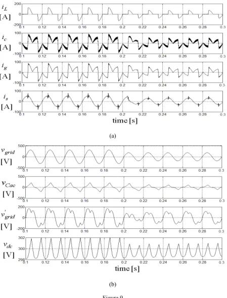
Fig. 2 shows the frequency responses of the hybrid LCL-filter corresponding to Eqs.(6)-(8), where the effect of damping resistance is also investigated. Fig. 2a indicates that the frequency response from inverter output Vo(s) to the grid-side current of the LCL-filter Ig(s) shows two resonant peaks, one in the low frequency range (185 Hz), another in the high frequency range (2.9 kHz). The resonant peak at low frequency range is caused by the LC resonance between the AC-side filter Cac and the total inductance L=Lg+Lc. And the resonant peak at the high frequency range is caused by the LC resonance between the RC-filter (Rd and Cd) and the total inductance L=Lg+Lc. The damping resistance is found to have negligible effect on the resonant peak in the lower frequency range. However, smaller damping resistance causes significant resonant peak in the high frequency range, which implies that insufficient damping might cause instability of the system at higher frequencies. Fig. 2b shows the frequency response of the hybrid LCL-filter section from Vo(s) to Ic(s). A similar resonant frequency in the low frequency range is observed.
Whereas Fig. 2b shows two resonant peaks in the high frequency range, one shows the characteristic of overshoot and another shows the feature of undershoot. Fig.
2b also shows that smaller damping resistance results in higher resonant peaks in the high frequency range, making the system vulnerable due to poor stability margin. Fig. 2c shows the frequency response from inverter output Vo(s) to the RC-filter brunch of the LCL-filter IRC(s). It shows that the resonant peak in the lower frequency range has an attenuation of -10dB, which implies that the lower frequency component generated by the VSI is damped in the RC-filter. However, the resonant peak in the high frequency range shows an attenuation of about 15 dB when the damping resistance is 0.05 Ω. It can also be inferred that smaller damping resistance results in current amplification at the RC-filter. Therefore, proper damping is mandatory to ensure the stable operation of the proposed system.
(a) (b)
(c) Figure 2
Frequency response of the hybrid LCL-filter under different damping resistances. (a) From inverter output Vo(s) to the grid-side current of the LCL-filter Ig(s); (b) From inverter output Vo(s) to the inverter-side current Ic(s); (c) From inverter output Vo(s) to the RC-filter brunch of the LCL-filter IRC(s)
3 Control System Design
The current control loop is a key element for APFs. The cascaded controller structure is adopted for the proposed hybrid APF, which contains inner current- loop and outer dc-voltage loop (Fig. 3). The inner current loop is responsible for fast harmonic tracking and the outer loop is used for balancing the active power flow of the APF through regulating the dc-bus capacitor voltage [26, 27].
The adaptive linear neural network (ADALINE) is utilized as a harmonic identifier, which recursively extracts the amplitude and phase angle of an individual harmonic component by using the Widrow-Hopf learning algorithm [28]. By using the ADALINE algorithm, the compensating current of the APF is
reconstructed; thus, the control bandwidth is effectively reduced, and the stability margin imposed by the current tracking algorithm is ensured over a wide operation range. To enhance the performance of the APF, the feed-forward control algorithm is devised by feeding the non-active component of the load current into the feed- forward loop, and the voltage drop across the AC-side capacitor Cac is utilized as the voltage feed-forward variable in the feed-forward control loop.
Figure 3
Control block diagram of the proposed hybrid LCL-filter based active power filter. (This figure is vertically presented for better clarity)
3.1 Harmonic Detection using Adaptive Linear Neural Network (ADALINE)
The most critical issues associated with APF control is that of finding an appropriate control algorithm, one which can obtain an accurate reference signal for control purposes, particularly when the load harmonics are time-varying [6-17].
Therefore, the performance of the APF strongly depends on the harmonic detection method [9-11]. To take advantage of the on-line learning capabilities of neural networks (NNs), the adaptive linear neural network (ADALINE) is utilized to estimate the time-varying magnitudes and phases of the fundamental and harmonic components from the source current and load current (Fig. 1) [6]. The motivation is to adopt a combined feed-forward and feedback control strategy for the proposed APF using ADALINEs as harmonic identifiers. For the sake of clarity, the background of ADALINE is briefly outlined herein [6, 28, 29].
An arbitrary signal Y(t) at the kth sampling time can be represented by the Fourier series expansion as:
0 0,1,2,3,
0 0
0,1,2,3,
( ) sin( ) ( )
( sin cos ) ( )
N
k n k n k
n N
n k n k k
n
Y t A n t t
a n t b n t t
ω ϕ ε
ω ω ε
= ⋅⋅⋅
= ⋅⋅⋅
= + +
= + +
∑
∑
(9)
where An and ϕn are correspondingly amplitude and the phase angle of the nth order harmonic component, and ε(tk) represents higher order components and random noise, and an, bn (n is integer) are also known as the Fourier coefficients, which can be calculated recursively using the least-mean-square (LMS) algorithm [30]. In other words, the Fourier coefficients can be estimated recursively by formulating the target signal Y(tk) as the inner product of the pattern vector Xk and weight vector Wk , which are defined as:
0 0 0 0
0 1 1 2 2
[1,sin , cos , ,sin , cos ]
[ , , , , ,..., , ]
k k k k k T
k k k k k k k T
k N N
X t t N t N t
W b a b a b a b
ω ω ω ω
⎧ = ⋅⋅⋅
⎪⎨
⎪⎩ = (10)
Therefore, the square error on the pattern Xk can be expressed as
2 2
2
1 1
( )
2 2
1( 2 )
2
k k kT k k
T T T
k k k k k k k k
d X W e
d d X W W X X W
ε = − =
= − +
(11)
where dk is the desired scalar output for the target signal Y(tk). The mean-square error (MSE) ε can be obtained by calculating the expectation of both sides of Eq.
(12), as:
1 2 1
[ ] [ ] [ ] [ ]
2 2
T T T
k k k k k k k k k
E E d E d X W W E X X W
ε = ε = − + (12)
where the weights are assumed to be fixed at Wk while computing the expectation.
The objective of the ADALINE is to find optimal weight vector Wˆk that minimizes the MSE of Eq. (13). When mean-square error ε is minimized, the weight vector Wˆ after convergence would be [6, 28, 29]:
0 1 1 2 2 T
ˆ [ , , , , ,..., N, N]
W = b a b a b a b (13)
Thus, the fundamental component and the nth order harmonic component of the measured signal can be obtained as:
1 1 0 1 0
0 0
( ) sin( ) cos( )
( ) sin( ) cos( )
k k k
n k n k n k
Y t a t b t
Y t a n t b n t
ω ω
ω ω
= +
⎧⎨ = +
⎩ (14)
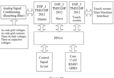
In this paper, the fixed-point digital signal processors (DSPs) from Texas Instruments (TI TMS320F2812) are adopted to implement the ADALINE-based estimation algorithm and the control algorithm for the APF. The phase and magnitude of the individual harmonic components, from the 3rd to the 25th order, are estimated for the higher convergence of ADALINE, but only the lower-order harmonics from 3rd to 19th order are selected in the current-loop control to save the computation resources. However, the selected harmonics can easily be extended.
The accurate and rapid estimation capability of ADALINE is crucial when selective harmonic compensation is adopted in current control for the purpose of reducing controller bandwidth, thus increasing system robustness and enhancing stability [28].
3.2 The Proposed Feedback plus Feed-forward Control Strategy
In this section, the feedback plus feed-forward control scheme are described consecutively. Firstly, the deadbeat control law for the average current control scheme is introduced by using the discrete domain representation of the LCL-filter model. Then, stability analysis of the closed-loop current control schemes under various parameter variation scenarios is presented. Finally, the feed-forward control loop, which achieves fast load disturbance compensation, is presented.
In the forthcoming derivations, the current in phase ‘a’ is analyzed for the sake of brevity. However, the same conclusions can also be applied for the other phases.
The load current in phase ‘a’ is represented by:
, 0 , 1
,1 0 ,1 0
, 0 , 0
2
( ) sin( )
sin( ) cos( )
[ sin( ) cos( )]
La La n La n
n
La PLL La PLL
La n La n
n
i t I n t
a t b t
a n t b n t
ω ϕ
ω ϕ ω ϕ
ω ω
∞
=
∞
=
= ∑ +
= + + +
+∑ +
(15)
where aLa,1=ILa,1cos(φLa,1-φPLL) and bLa,1=ILa,1sin(φLa,1-φPLL) represent the amplitude of the fundamental active and reactive component of the nonlinear load current, and φPLL represents the initial phase angle of the phase-locked-loop (PLL) [28, 29], which is synchronized with the fundamental frequency component of the grid voltage. And ILa,n and φLa,n(n>1, n is integer) represent the amplitude and phase angle of the nth order harmonic component of the load current, respectively. The parameters aLa,n and bLa,n (n>1, n is integer) represent the weights of the individual harmonic component obtained from the ADALINE. The individual harmonic component can be reconstructed using Eq. (15) if the weights aLa,n and bLa,n (n is integer) are precisely calculated. Similarly, the source-side current in phase ‘a’
supplied by the distribution system is represented as:
,1 0 ,1 0
, 0 , 0
2
( ) sin( ) cos( )
[ sin( ) cos( )]
sa sa PLL sa PLL
sa n sa n
n
i t a t b t
a n t b n t
ω ϕ ω ϕ
ω ω
∞
=
= + + +
+∑ + (16)
where asa,1= Isa,1cos(φsa,1-φPLL) and bsa,1=Isa,1sin(φsa,1-φPLL) represent the amplitude of the fundamental active and reactive component of the source-side current, and Isa,n and φsa,n (n>1, n is integer) represent the amplitude and phase angle of the nth order harmonic component of the source-side current, respectively. The parameters asa,n and bsa,n (n is integer) represent the weights of the individual harmonic component obtained from a separate ADALINE block in the feedback loop (Fig. 3). To achieve the feedback current tracking control, the fundamental reactive component and the selected harmonic components are utilized as the reference current for the APF. Furthermore, the output of the voltage-loop controller ΔIp, after being multiplied by a unit sinusoidal signal synchronized with the grid voltage by using PLL, is added to the feedback current to compensate for the power loss of the inverter [6-19]. Therefore, the compensating current of the APF in the feedback loop is represented as:
,1 0 , 0 , 0
, 3
0
( ) { cos( ) [ sin( ) cos( )]}
sin( )
ref N
sa PLL sa n sa n
ga fb
n
p PLL
i t b t a n t b n t
I t
ω ϕ ω ω
ω ϕ
= − + + ∑= +
+Δ +
(17)
Note that a finite number of harmonics is selected in Eq. (17), since only a limited number of harmonics are processed in the ADALINE-based harmonic estimation scheme due to the limited computational load, constrained by the DSP.
Figure 4
Principle of current tracking control scheme: (a) Geometrical interpretation for deriving the average current during one PWM period; (b) Schematic of the voltage source inverter (VSI) and its output
voltage
3.2.1 Deadbeat Control Scheme for the Feedback Current Control Loop To simplify the control effort for the proposed hybrid APF, the deadbeat control scheme is adopted in the feedback closed-loop for reference current tracking. Only the LCL-section of the hybrid APF is used to derive the deadbeat control law. The AC-side capacitor voltage, on the other hand, is regulated by controlling the injection current of the LCL-filter. Moreover, the RC-filter brunch of the LCL- filter section, adopted for high frequency switching ripple attenuation and stability enhancement, shows little impact on the low frequency range below 2 kHz (Fig.
2a). Hence, the effect of the RC-filter is neglected when deriving the deadbeat control law for the sake of simplicity. Therefore, the degree of freedom of the control system for the hybrid APF is significantly reduced.
Utilizing the concept of the reduced order model for the LCL-filter, the deadbeat current control law for the inner current loop is derived herein. Firstly, the differential equation for the inductor current across LCL-filter section is represented as:
( )
- -
grid Cac o g c
v v v L L di
= + dt (18)
where parameters νgrid, νCac and νo represent the grid side voltage, the AC- capacitor voltage and output voltage of the voltage source inverter, respectively. In order to derive the discrete domain representation of Eq. (18), the operation
principle of the inverter under different switching patterns is given by Fig. 4. It can be observed that, when the switches G1 and G4 are switched on, and the switches G2 and G3 are turned off, the output voltage of the inverter is vdc, and then the inverter current undergoes a falling stage, according to the direction of current defined in Fig. 1. When the switches G1 and G4 are switched off, and switches G2 and G3 are switched on, the output voltage of VSI would be -vdc, which results in a rising stage of the inverter current (Fig. 4a-b). Therefore, Eq.
(18) can be rewritten in the discrete form using piecewise linear representation as:
[ ] - [ ] - [ ] [( ) ] - [ ]
2 2
[ ] - [ ] [ ] [( 1- ) ] - [( ) ] (1- )
2 2
[ ] - [ ] - [ ] [( 1) ] - [( 1- ) ]
2 2
grid Cac dc
g s g s s
g c
grid Cac dc
g s g s s
g c
grid Cac dc
g s g s s
g c
v k v k v k
d d
i k T i kT T
L L
v k v k v k
d d
i k T i k T d T
L L v k v k v k
d d
i k T i k T T
L L
⎧ + = ⋅
⎪ +
⎪⎪ +
⎪ + + = ⋅
⎨ +
⎪⎪
⎪ + + = ⋅
⎪ +
⎩
(19)
where d in Eq. (19) is the abbreviation of d[k], representing the duty cycle of the kth control period. The grid voltage and AC capacitor voltage are assumed to be constants during one PWM cycle (quasi-steady-state model) in discrete equations.
After mathematical manipulations of Eq. (19), the duty ratio of PWM signal at the kth control period is obtained as:
( ){ [( 1) ] - [ ]} [ ] [ ] - [ ]
[ ] -
2 [ ] 2 [ ]
g c g s g s dc grid Cac
dc s dc
L L i k T i kT v k v k v k
d k v k T v k
+ + +
= + (20)
In order to track the reference signal and achieve deadbeat control, the current at (k+1)th sampling interval ig[(k+1)Ts] should be replaced by the reference signal at the next sampling cycle [26, 31]. Nevertheless, in the proposed hybrid APF, the resetting filters are adopted at the sampling stage, and hence the instantaneous quantities cannot be directly obtained at kth and (k+1)th sampling instants. On the contrary, all the sampling signals, i.e., the voltages and currents, are the average quantities of the previous period. Therefore, the current tracking scheme should be modified to account for the average quantities, and hence the theoretical derivation of the average current during the kth control period is given herein.
Referring to Fig. 4a, it can be deduced that, during the switching on/off processes of the power electronic switches, the output current during one control period undergoes rising and falling stages according to the switching patterns of the switches. Therefore, the average current can be obtained by dividing the total shadowed area denoted as S1, S2 and S3 by the control period Ts. As shown in Fig.
4a, the slopes of the current i(t) during one PWM control period are denoted as:
1 3
2
[ ] - [ ] - [ ] [ ] - [ ] [ ]
grid Cac dc
g c
grid Cac dc
g c
v k v k v k k k
L L v k v k v k
k L L
⎧ = =
⎪ +
⎪⎨ +
⎪ =⎪ +
⎩
(21)
The shadowed area denoted as S1, S2 and S3 in Fig. 4a can be derived as:
1 1
2 1 2
3 1 2
1{2 [ ] }
2 2 2
1{2 [ ] (1 ) } (1 )
2
1{2 [ ] 3 2 (1 ) }
2 2 2
g s s s
g s s s s
g s s s s
d d
S i kT k T T
S i kT k dT k d T d T
d d
S i kT k T k d T T
⎧ = + ⋅
⎪⎪
⎪ = + + − ⋅ −
⎨⎪
⎪ = + ⋅ + − ⋅
⎪⎩
(22)
Therefore, the average inverter current of the kth control period can be derived as:
1 2 3
[ ]
g s
s
S S S
i kT T
+ +
= (23)
Therefore, from Eqs. (22) and (23), the instantaneous current at the (k+1)th sampling instant can be rewritten as:
{ [ ] [ ] - [ ]} 2 [ ]
[( 1) ] [ ]
2( )
dc grid Cac s s dc
g s g s
g c
v k v k v k T dT v k i k T i kT
L L
+ −
+ = +
+ (24)
Hence, the duty cycle can be rewritten in terms of the average current of the kth sampling period as:
( ){ [( 1) ] - [ ]} [ ] [ ] - [ ]
[ ] -
[ ] 2 [ ]
g c g s g s dc grid Cac
dc s dc
L L i k T i kT v k v k v k
d k v k T v k
+ + +
= + (25)
In Eq. (25), the term L/Ts is denoted as the current controller gain derived from the deadbeat control law. It is interesting to notice from Eq. (20) and Eq. (25) that the deadbeat control law for the average current tracking control and the instantaneous current tracking control have similar expression. However, the controller gain, denoted by L/Ts, for the current tracking error in Eq. (25) of the average current tracking scheme is twice the value of the instantaneous current tracking scheme, which shows the superior performance for the proposed scheme; i.e., the adoption of resetting filter is helpful in increasing the current controller gain, thus increasing the tracking dynamics for the reference compensation current of the APF.
Nevertheless, the aforementioned deadbeat control scheme is based on the reduced order model of the LCL-filter, where the RC-filter is neglected at the modeling stage. Hence, the performance of the current tracking scheme may be imperfect
due to model mismatch and parameter uncertainty. Therefore, the stability analysis of the current control scheme is rigorously studied to ensure the stable operation of the APF. In the forthcoming subsection, the RC-filter is incorporated into the mathematical manipulations and the selection of the current controller gain is discussed with respect to the stability requirement.
3.2.2 Root Locus Analysis of the Grid-side Current Tracking Scheme This subsection presents the performance of the grid-side current (ig) tracking scheme by using the closed-loop root locus plots and the open-loop impulse responses. The plant model under this scenario can be obtained by deriving the open-loop transfer function from the inverter output to the grid-side current of the LCL-filter section:
0 0
, 3 2
0 0 0 0 0 0 0 0 0
( ) 1
( ) ( )
d d
g plant
g c d d d g c g c
R C s
G s
L L C s R C L L s L L s
= +
+ + + + (26)
The current loop transfer function Gg,cc(s) is simply represented by a proportional gain Kcc, and the transfer function of the delay due to PWM generation and computational delay (Td) is expressed as:
, ( ) sTd
g delay
G s =e− (27)
Hence the open loop transfer function of the grid-side current tracking control algorithm can be represented by:
, , , ,
0 0
3 2
0 0 0 0 0 0 0 0 0
( ) ( ) ( ) ( )
1
( ) ( )
d
g open g cc g plant g delay
sT d d
cc
g c d d d g c g c
G s G s G s G s
R C s
K e L L C s R C L L s L L s
−
=
= +
+ + + +
(28)
Therefore, the closed-loop transfer function of the grid-side current tracking control scheme can be derived as:
, 0 0
, 3 2
, 0 0 0 0 0 0 0
0 0 0 0
( ) ( 1)
( ) 1 ( ) { ( )
( ) }
d
d d
g open cc sT d d
g close
g open g c d d d g c
sT sT
cc d d g c cc
G s K e R C s
G s
G s L L C s R C L L s
K R C e L L s K e
−
− −
= = +
+ + +
+ + + +
(29)
It should be noted that, to achieve an optimal dynamic performance of the proposed hybrid APF, the selection of the current loop controller should be rigorously studied. If the gain is selected too small, the dynamic response of the current tracking will be sluggish. On the other hand, if the current loop gain is too high, the stability constraint of the closed-loop control will be violated. Hence the current loop gain will be carefully studied in the subsection by using discrete domain representation of the closed-loop transfer function under various parameter variation scenarios, which will be discussed herein.
Referring to Eq. (29), the closed-loop transfer function of the current loop tracking control under nominal system parameters can be rewritten in the discrete domain (z-domain) as:
2
, 4 3 2
(0.08836 0.09784 0.004811) ( ) { 0.9407 (0.08836 0.2419)
(0.09784 0.3012) 0.004811 }
cc g close
cc
cc cc
K z z
G z
z z K z
K z K
+ −
= − + +
+ − −
(30)
where Td is assumed to be one control period (Ts=100μs). The closed-loop root locus plot and open-loop impulse response of the grid-side current control scheme under nominal system parameters is illustrated by Fig. 5a. It can be observed that the closed-loop system would be unstable when the current controller gain exceeds 5.6. It is interesting to notice that this stability margin is lower than the controller gain directly derived from the deadbeat control low. This gain limit should be satisfied in the practical system to ensure closed-loop stability, as discussed in the simulation and experimental results. Moreover, it can be observed from Fig. 5a that the open-loop impulse response shows an overshoot of 0.18 p.u with the response time of 1.2 millisecond. In order to investigate the robustness of the presented hybrid APF and the control scheme, the influence of parameter variations is also rigorously studied herein by taking into account the variation of interfacing inductances, the control delay and the RC filter parameter variations.
It should be noted that the interfacing inductances may deviate from their nominal values in practical systems due to the variation of the operational conditions, humidity and temperature deviation. Hence the influence of inductance variations is considered here by changing the grid-side inductance to 0.8 p.u and converter side inductance to 1.2 p.u. Under this condition, the closed-loop transfer function of the grid-side current tracking scheme in discrete domain can be derived as:
2
, 4 3 2
(0.09322 0.1047 0.00515) ( ) { 0.9617 (0.09322 0.2731) (0.1047 0.3114) 0.00515 }
cc g close
cc
cc cc
K z z
G z
z z K z
K z K
+ −
= − + +
+ − −
(31)
The closed-loop root locus plot and open-loop impulse response of the grid-side current tracking scheme under inductance variations is illustrated by Fig. 5b. It can be observed that the closed-loop system would be unstable when the current controller gain exceeds 5.15, which is lower than the case of the nominal system parameters. Besides, it can be observed from Fig. 5b that the open-loop impulse response shows an overshoot of 0.195 p.u with the response time of 1.2 millisecond. Next, we consider the effect of the control delay on the performance of the current tracking control, which is associated with PWM generation and computational delay, etc. Considering the control delay as 1.5Ts, then the closed- loop transfer function of the current tracking algorithm is derived as:
3 2
, 5 4 3
2
(0.02253 0.1347 0.02834 0.00414) ( ) { 0.9407 (0.02253 0.2419)
(0.1347 0.3012) 0.02834 0.00414 }
cc g close
cc
cc cc cc
K z z z
G z
z z K z
K z K z K
+ + −
= − + +
+ − + −
(32)
The closed-loop root locus plot and open-loop impulse response of the grid-side current tracking scheme corresponding to the variation of control delay is illustrated by Fig. 5c. It can be observed that the closed-loop system would be unstable when the current controller gain exceeds 4.87, which is lower than the case of the nominal system parameters. Besides, it can be observed from Fig. 5c that the open-loop impulse response shows an overshoot of 0.17 p.u with the response time of 1.2 millisecond, which is almost the same as the case of the nominal system parameters. It is also found that a longer delay would not only deteriorate the stability of the closed-loop system, but would also significantly hamper the quality of the output voltage waveform, which would result in poor precision of the current tracking algorithm. However, as discussed in the experimental results, the control delay does not have a significant effect on the performance of the system since the ADALINE-based harmonic estimation algorithm was adopted to generate the reference current for the current loop controller. Hence the control delay can be compensated for by shifting the reference compensation current of the APF by one sampling period, which can be easily achieved by adding Δθn (Δθn=ωnTs=2πf0nTs, n is the harmonic order) to the phase angle of the individual harmonic component by modifying the sin(nω0t) and cos(nω0t) into sin(nω0t+Δθn) and cos(nω0t+Δθn) in the reconstruction process of the ADALINE-based harmonic estimation algorithm.
Next, we consider the effect of the RC-filter parameters on the performance of the current loop tracking algorithm by changing the filtering capacitance and the damping resistance, respectively. If the filtering capacitance of the RC-filter is modified to Cd=5 μF, then the closed-loop transfer function of the current tracking control algorithm is derived as:
2
, 4 3 2
(0.1391 0.1296 0.04588) ( ) { 0.05781 (0.1391 0.7566)
(0.1296 0.3012) 0.04588 }
cc g close
cc
cc cc
K z z
G z
z z K z
K z K
+ +
= + + −
+ − +
(33)
The closed-loop root locus plot and open-loop impulse response of the grid-side current tracking control with the variation of filtering capacitance is illustrated by Fig. 5d. It can be observed that the closed-loop system would be unstable when the current controller gain exceeds 7.66, which is much higher than the case of the nominal system parameters. Moreover, it can be observed from Fig. 5d that the open-loop impulse response shows an overshoot of 0.144 p.u with the response time of 1.1 millisecond, which is remarkably lower than the case of nominal system parameters. It is found that the smaller the filtering capacitance, the higher the stability margin and the faster the dynamic response of the current tracking
control algorithm can be achieved. Nevertheless, smaller filtering capacitance would result in poor attenuation of higher order switching harmonics. Therefore, a compromise should be achieved between the filtering efficiency and the closed- loop stability constraint. Next, the effect of the damping resistance on the closed- loop current tracking control is examined by changing the damping resistance Rd
to 0.1Ω, and then the closed-loop transfer function can be derived as:
2
, 4 3 2
(0.05958 0.189 0.05182) ( ) { 0.6889 (0.05958 0.6306)
(0.189 0.9418) 0.05182 }
cc g close
cc
cc cc
K z z
G z
z z K z
K z K
+ +
= − + +
+ − +
(34)
The closed-loop root locus plot and open-loop impulse response of the grid-side current tracking control scheme with the variation of damping resistance is illustrated by Fig. 5e. It can be observed that the closed-loop system would be unstable when the current controller gain exceeds 5.29, which is lower than the case of the nominal system parameters. Besides, it can be observed from Fig. 5e that the open-loop impulse response shows an overshoot of 0.23 p.u with the response time of 18 millisecond, which is significantly higher than the case of the nominal system parameters. It is found that a smaller damping resistance would result in a smaller stability margin and a prolonged dynamic response of the current tracking control scheme. On the other hand, however, the reduced damping resistance results in a higher damping of higher order switching harmonics of the inverter, as demonstrated in Fig. 2a. Therefore, a compromise must be achieved between the stability constraint and the switching ripple attenuation for practical systems. Table 2 shows the summery of the stability margin and dynamic response of the grid-side current tracking control scheme, where the results obtained under the nominal system parameters and parameter variation scenarios are presented. In the forthcoming subsection, a similar analysis is provided for the closed-loop locus diagrams and open-loop impulse responses of the current regulation scheme based on the converter-side tracking control scheme.
Table 2
Summary of the stability margin and dynamic response of the grid-side current tracking scheme Case Marginal gain (deg) Overshoot (pu) Response time (ms)
1 5.6 0.18 1.2
2 5.15 0.195 1.2
3 4.87 0.17 1.2
4 7.76 0.144 1.1
5 5.29 0.23 18
(a)
(b)
(c)
(d)
(e) Figure 5
The closed-loop root locus diagrams and the open-loop impulse responses of the current regulation algorithm based on the grid-side current (ig) tracking control scheme. (a) Root locus and impulse response under nominal parameters; (b) Root locus and impulse response under inductance variations;
(c) Root locus and impulse response under different control delay (Td=1.5Ts); (d) Root locus and impulse response under different RC-filter capacitance Cd; (e) Root locus and impulse response under
different RC-filter resistance Rd
3.2.3 Root Locus Analysis of the converter-side Current Tracking Scheme This subsection presents the performance of the converter-side current (ic) tracking scheme by using the closed-loop root locus plots and the open-loop impulse responses. The plant model under this scenario can be obtained by deriving the open-loop transfer function from the inverter output to the converter side current of the LCL-filter section: