FINITE PLASTIC DEFORMATION William Prager

FINITE PLASTIC DEFORMATION William Prager

I. Introduction 63 1. Elastic Deformation. Viscous and Plastic Flow 63

2. Plastic-Rigid Solids 65 II. Flow of Perfectly Plastic Solids 66

1. Fundamental Concepts 66 2. Yield Condition 67 3. Flow Rule 70 4. Principle of Maximum Local Energy Dissipation 72

5. Theory of Plane Plastic Flow 76 6. Examples of Plane Plastic Flow 80

a. Necking in Tension 80 b. Sheet Extrusion 82 c. Wedge Indentation 85 d. Bulge Test 88 III. Flow of Work-Hardening Plastic Solids 89

IV. Flow of Visco-Plastic Solids 93

Nomenclature 96 I. Introduction

1. E L A S T I C D E F O R M A T I O N . V I S C O U S AND P L A S T I C F L O W

The mechanical behavior of solids is extremely complex. Even if the necessary empirical information were available, it would probably be diffi- cult to construct a single mathematical model representing such varied phenomena as instantaneous elastic deformation, elastic aftereffect and hysteresis, creep, and plastic flow, under combined stresses. Anyhow, such a model would be too unwieldy to furnish a practical basis for the treatment of technological problems involving stresses and strains in solids. Simpler models must be used, representing only those mechanical properties that are essential to the considered problem. Furthermore, the need for mathe- matical simplicity often dictates far-reaching idealizations in the mathe- matical description of the properties that are to be incorporated in the model.

The Hookean elastic solid and the Newtonian viscous liquid are the best known models of this kind. They are mathematical abstractions, as devoid of physical reality and yet as useful tools for dealing with physical realities as are the geometrical point and line. This article is concerned with those

63

models in mechanics of continua that lend themselves to the discussion of large plastic deformations. Most important amongst these are the perfectly plastic solids (Tresca solid, Mises solid).

Many concepts that will be used in the following can be explained with reference to elastic solids and viscous liquids. The term liquid indicates that the state of stress at a generic point reduces to a state of hydrostatic pressure when the substance is at rest. In a solid, stresses other than mere hydrostatic pressure can be maintained during rest. The term viscous implies that the stress depends on the speed of deformation; absence of vis- cosity effects is indicated by the term inviscid.

An elastic solid is a conservative system: the mechanical energy used to produce a deformation is stored in the deformed solid and can be regained upon unloading. A viscous liquid is a dissipative system: the mechani- cal energy used to overcome the internal friction that opposes deformation is converted into heat.

The finite deformations of an elastic solid constitute a topic of consider- able mathematical difficulty. To avoid this difficulty, most investigations concerning elastic solids are restricted to infinitesimal deformations. For a viscous liquid, on the other hand, the study of finite deformations does not present particular mathematical difficulties: even problems that can be treated with elementary means, for instance, the Poiseuille flow through a tube of circular cross section, involve finite deformations. The reason for this striking difference between elastic solids and viscous liquids is the following: the mechanical behavior of an elastic solid is defined in terms of stress and strain, but that of a viscous liquid is defined in terms of stress and velocity strain. In specifying strain, we compare the deformed state to some reference state, usually the stress-free state. When the devia- tion between these states is finite, the mathematical formulas defining strain become rather complex. In specifying velocity strain, on the other hand, we compare the states at the instants t and t + dt. The deviation between these states is infinitesimal, and the mathematical complication encountered for finite strain does not arise.

The state of stress in an elastic solid is related to the instantaneous state of deformation; in a viscous liquid, and also in the plastic solids considered in this article, the state of stress is related to the instantaneous state of ow. In the following, the terms viscous flow and plastic flow are used in a special sense, which should be clearly understood. Both types of flow involve dissipation of energy and lead to permanent deformations. For vis- cous flow, the mechanical energy dissipated in producing a given deforma- tion depends on the speed of deformation, whereas in plastic flow the energy dissipation is independent of the speed. In actual solids, both types of flow

may occur simultaneously; the relative importance of their contributions to the permanent deformation depends on the temperature and stress in- tensity, high temperatures and low stresses favoring viscous flow.

The mathematical analysis of permanent deformations is greatly sim- plified when the two types of flow are considered separately. Except for a brief section on visco-plastic flow (section IV), this article is con- cerned with plastic flow only.

2. PLASTIC-RIGID SOLIDS

The yield limit of a plastic material indicates the stress level below which plastic deformation is absent or insignificant. Some materials (for instance, mild steel) possess a sharply defined natural yield limit. For most materials, however, the yield limit is conventional: plastic deforma- tions are ignored until they exceed a critical magnitude that depends on the problem under consideration.

Technological problems concerning stresses and strains in plastic solids fall into two groups, which may be labeled problems of small elastic-plastic deformations and problems of plastic flow. In problems of the first kind, the deformations of the plastic portions of the solid are restricted by the fact that adjacent portions of the solid have not yet reached the yield limit and hence are capable of small elastic deformations only. The presence of elasti- cally stressed portions of the solid is not excluded in problems of the second kind, but the geometry of these portions is assumed to be such that they cannot prevent large deformations of the plastic portions. In a grooved ten- sion specimen, for instance, plastic deformation begins at the groove, but the extension of the specimen is controlled by the elastic core until the plastic portion extends all the way across the specimen.

Different mathematical simplifications are appropriate in each case. In problems of small elastic-plastic deformations, the strains may be treated as infinitesimal, but both elastic and plastic strains must be considered, be- cause they are of the same order of magnitude. In problems of plastic flow, on the other hand, the strains cannot be treated as infinitesimal, but the elastic strains are usually so much smaller than the plastic strains that they may be neglected. In fact, tremendous mathematical difficulties can be avoided only if the elastic strains are neglected: even though the elastic strains are small, their consideration would imply the use of the stress-free state as the reference state for the formulation of both, the elastic and the plastic stress-strain laws. In the resulting mathematical theory, the difficul- ties inherent in the consideration of finite strains would be combined with the difficulties springing from the essential nonlinearity of plastic stress- strain laws. If the elastic strains are neglected, however, a plastic stress-

strain law can be used that involves velocity strain rather than strain;

the complications resulting from finite strains are then avoided in the same manner as in the theory of viscous liquids.

Neglecting the elastic strains is equivalent to considering the material as rigid as long as the stresses remain below the yield limit. The theory of large plastic deformations that is to be presented in this article thus is concerned with plastic-rigid solids. Perfectly plastic and work-hardening solids will be considered. A perfectly plastic solid is capable of plastic flow under constant stress; in a work-hardening solid, however, the stress in- tensity must be increased continually if plastic flow is to be maintained.

II. Flow of Perfectly Plastic Solids 1. FUNDAMENTAL CONCEPTS

With respect to fixed rectangular Cartesian axes x, y, and z, the state of stress at a point of the solid is specified by the components p^x, p^y , p^z, Pxy , Vyz > ^{a n}d Pzx, of the stress tensor. Alternatively, the state of stress may be specified by the principal stresses p\, p², and p³, and three Eulerian an- gles defining the orientation of the principal axes of stress. Similarly, the rate of strain is specified by the components D^x , D^y , D^z, D^iy , D^yz, and D^zx , of the strain-rate tensor or by the principal strain rates D\ , D², and Z)³, and three angles defining the orientation of the principal axes of the rate of strain. In terms of the velocity components u, v, and w, the components of the strain rate are defined by

D . - 2 * Λ . « £ + ? (1) dx dx dy

and the relations obtained from (1) by simultaneous cyclic permutation of x, y, z and u, v, w.

The solids considered in this chapter are incompressible. Thus,

Dx + Dy + Dz = D1 + D, + D3 = ~ + ~ + p- = 0 (2) ax dy dz

It is often convenient to decompose the stress tensor into a hydrostatic and a deviatoric part. Both parts have the same principal axes as the stress tensor itself; the principal values of the hydrostatic part are all equal to the mean normal stress:

V = H(P* + Vy + p^z) = Η(ρι + Ρ2 + pz) (3) The principal values of the deviatoric part or stress deviation are

Pi = Pi ~ P pi = Pi - P Pz = Pz - p (4) With respect to arbitrary rectangular axes x, y, and z, the stress deviation

has the components

V* = P* - P Vy = Vv - P Vz = Vz - p)

( 5 ) Pxy — Pxy Pyz — Pyz Pzx — Pzx J

In plastic flow with the principal strain rates Di, D2, Dz and the principal stresses pi, p2, pz, mechanical energy is dissipated at the rate

ß = H ( p A + P2Ö2 + p3D3) (6)

per unit volume. Alternative expressions for δ are δ = MPI'DI + p2fD2 + pz'Dz)

δ = %(p*Dx + pyDy + p2Dz) + pxyDxy + pyzDyz + p2XDzx (7) S = J4(P*D* + PyDy + Pz'Dz) + p'xyD^ + p^Z)^ + pL#2x

The condition of incompressibility (2) and equations (4) and (5) have been used to effect the changes from (6) to the first line of (7) and from the sec- ond to the third line of (7).

2. YIELD CONDITION

The mechanical behavior of the perfectly plastic solids considered in this section is characterized by the yield condition and the flow rule. The yield condition defines the stress level at which significant plastic deformation becomes possible; for lower stresses the solid is treated as rigid. For states of stress at the yield limit, i.e., states of stress satisfying the yield condition, the flow rule establishes relations between strain rate and stress.

In an isotropic perfectly plastic solid, the principal axes of strain rate and stress coincide. Moreover, the yield condition and the flow rule, for- mulated in terms of principal stresses and principal strain rates, are inde- pendent of the orientation of the principal axes in the solid.

To discuss possible yield conditions for isotropic, perfectly plastic solids, it is convenient to represent a state of stress with the principal stresses pi, p2, and p3, by the point in stress space that has the rectangular Car- tesian coordinates px, p2, and p3. In the following, this point will be called the stress point.

The plane in stress space that has the equation px + p2 + pz = 0 will be called the deviatoric plane, and the line through the origin that is perpen- dicular to this plane will be called the hydrostatic axis of stress space. Stress points on this axis represent purely hydrostatic states of stress, which have equal principal stresses, and stress points in the deviatoric plane represent purely deviatoric states of stress, which have vanishing mean normal stress.

To the decomposition of the stress tensor into its hydrostatic and deviatoric

parts [see equation (4)] there corresponds the decomposition of the radius vector of the stress point into a component along the hydrostatic axis and a component in the deviatoric plane.

The yield surface is the locus of all stress points that represent states of stress at the yield limit. In extrapolation of experimental results, it is usually assumed that the yield surface is a cylinder or prism with generators parallel to the hydrostatic axis. This amounts to assuming that states of stress below the yield limit cannot be raised to the yield limit by the super- position of purely hydrostatic states of stress. As a consequence of this as- sumption, the shape of the yield surface is determined by its cross section in the deviatoric plane.

F I G . 1. F I G . 2.

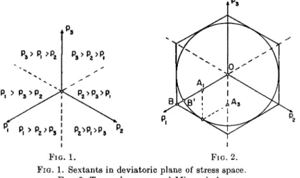
FIG. 1. Sextants in deviatoric plane of stress space.

FIG. 2. Tresca hexagon and Mises circle.

The projections of the positive coordinate axes in stress space on the deviatoric plane form angles of 120 deg. with each other, and the projec- tions of the negative coordinate axes bisect these angles. The deviatoric plane is thus divided into the sextants shown in Fig. 1. Since the order of numbering the principal axes has no physical meaning, the shape of the cross section of the yield surface in one of these sextants determines the shape in all other sextants by symmetry with respect to the sextant boun- daries.

The most frequently used yield conditions are due to Tresca¹ and Mises.² The yield surface for Tresca's yield condition is a regular hexagonal prism, and the yield surface for the yield condition of Mises is the circular cylinder inscribed to the Tresca prism. The intersections of these yield surfaces with

1 H. Tresca, Mem. pres. par div. savants 18, 733 (1868).

2 R. von Mises, Goettinger Nachr., Math. Phys. Klasse, p. 582 (1913).

the deviatoric plane are shown in Fig. 2. The common points of the hexagon and the circle in this figure correspond to states of pure shear such as the state defined by p\ = k,p2 = 0, p3 = — fc, where k is the yield stress in pure shear. In Fig. 2 this state of stress is represented by the point A. It should be noted that each of the segments OA\ and OAz in Fig. 2 has the length k/ \ / 3 ; the common length of the corresponding segments on the pi and p%

axes in stress space is k. The corners of the Tresca hexagon represent the deviatoric states of stress associated with states of uniaxial tension or compression. The corner B in Fig. 2, for instance, is associated with the state of uniaxial tension defined by p\ = 2k, p2 = p* = 0. The corresponding point B' on the Mises circle is associated with the state of uniaxial tension specified by pi = k \/3> p2 = p* = 0. The yield conditions of Tresca and Mises thus differ by about 15% in their predictions for the yield limits in uniaxial tension or compression while agreeing in their predictions for the yield limits in pure shear.

If the largest principal stress is denoted by pmax and the smallest by Pmin , Tresca's yield condition is

Pmax — Pmin = 2k (8)

It states that in plastic flow, the maximum shearing stress has the constant value k. Since any one of the principal stresses p\, p2, and p3 may be the largest, and any one of the two remaining principal stresses may in turn be the smallest, equation (8) furnishes the six faces of the Tresca prism.

In terms of the principal components (4) of the stress deviation, Mises' yield condition is

p? + p? + P? = 2fc² (9)

The advantage of this condition over that of Tresca is that it substitutes a single analytical expression for the six equations of the faces of the Tresca prism. Moreover, unlike the Tresca condition, the Mises condition is readily expressed in terms of the stress deviation components with respect to arbitrary rectangular axes x, y, and z. In fact, equation (9) is equivalent to³

ρΊ + Py² + V? + 2(/C + P'vl + Vl) = 2k² (10) The Mises condition was originally suggested as a mathematically conven-

ient approximation to the Tresca condition, which was then believed to represent the physical facts. When it was found, however, that for many metals Mises' condition agrees better with the experimental data than Tresca's condition, the question of the physical significance of the Mises

3 See, for instance, W. Prager and P. G. Hodge, Jr., "Theory of Perfectly Plastic Solids," p. 20 fif. Wiley, New York, 1951.

FIG. 3. Yield stress in com- pression exceeding that in ten- sion.

condition arose. Various interpretations have been given; the best known of these uses Nadai's⁴ concept of the octahedral shearing stress.

Consider any plane that has the same orientation with respect to the principal axes as a face of a regular octahedron has with respect to the axes of the octahedron.

The shearing stress transmitted across such a plane is called the octahedral shearing stress; the left-hand sides of (9) and (10) turn out to be proportional to the square of the octahedral shearing stress, the factor of proportionality being 3.

Actually, such physical interpretations tend to obscure the real reason for the importance of Mises' yield condition: this importance stems from the fact that this condition defines the simplest yield surface with straight generators parallel to the hydrostatic axis and with a cross section in the deviatoric plane that is symmetric with respect to the sextant boundaries.

Even if the agreement with experimental results had been much worse than it turned out to be, this yield condition would have played an important role in the theory of plasticity on account of its mathematical simplicity.

The Mises circle and the Tresca hexagon in Fig. 2 are symmetrical with respect to the origin 0. This symmetry indicates that the yield stresses in simple tension and simple compression have the same intensity.

The opinion is occasionally expressed in the literature that isotropy requires this sort of symmetry. This is not the case, however; Figure 3 shows the cross section of a prismatical yield surface for an isotropic solid that has a higher yield stress in compression than in tension.

3. FLOW RULE

The yield condition characterizes the states of stress at the yield limit.

For any such state of stress, the flow rule describes the possible states of plastic flow. Since the perfectly plastic solids considered here are isotropic, the principal axes of the strain rate coincide with those of the stress, and the flow rule reduces to a set of relations between the principal strain rates and the principal stresses. Since the considered solids are inviscid, the flow rule specifies the principal strain rates at most to within an arbitrary factor λ. This factor is restricted in sign, because the strain rate associated with a given state of stress at the yield limit must be such that mechanical energy

4 A. Nadai, J. Appl Phys. 8, 205 (1937).

is dissipated in plastic flow. In the following, flow rules will always be writ- ten so that the factor λ is nonnegative.

Principal strain rates specified to within an arbitrary nonnegative factor will be said to define a flow mechanism. In stress space, the flow mechanism associated with a given point on the yield surface may be represented by the ray issuing from this point and having direction cosines with respect to the axes in stress space that are proportional to the principal strain rates, the factor of proportionality being nonnegative. To formulate a flow rule then means associating such rays with all points on the yield surface.

In the following, it will be assumed that the yield surface is cylindrical or prismatical with generators parallel to the hydrostatic axis of stress space and that the rays associated with stress points on the same generator are parallel to each other. This means that the flow mechanism associated with a given state of stress depends only on the stress deviation but not on the mean normal stress. On account of the condition of incompressibility, equation (2), the rays associated with the various points of the yield surface must all be parallel to the deviatoric plane. The geometrical dis- cussion of the flow rule may therefore be restricted to the deviatoric plane.

The yield surface is represented by its intersection with this plane. With each point of this intersection, which is called the yield locus, the flow rule associates a ray in the plane of this locus.

The most widely used flow rule was developed by L6vy⁵ and v. Mises.² With the generic point P on the yield locus this flow rule associates the ray that has the direction of the radius vector OP. In terms of the principal components of the strain rate and the stress deviation, the flow rule of L£vy and v. Mises is

Di = λρΛ D2 = λρ2', JD« = λρ/; λ ^ 0 (11) Equations (11) are reminiscent of the relations that exist in a perfectly elastic solid between the principal strain rates and the principal com- ponents of the stress deviation, but there is an important difference be- tween these relations and equations (11). In an elastic solid, the common ratio between each principal strain and the corresponding principal com- ponent of the stress deviation is the reciprocal of the shear modulus, a physical constant characterizing the mechanical behavior of the solid. The factor λ in equations (11), however, is not a physical constant. In fact, this factor can be eliminated from equations (11) by means of the yield condi- tion. For brevity, we shall discuss this elimination only for the Mises yield condition. Substitution of (11) into (9) furnishes

X = l ^ ( Z )

+ Z )

+ D

) J

(12)

6 M. Lövy, Compt. rend. 70, 1323 (1870).

Equations (11) can therefore be written in the form

Di _ Pi Dt Pi

\^χΛΦΐ + W + Ö3²)]¹'² k ' \y2{DJ + Di + Da²)]¹'² k ' Di _ p / [M(öi² + Di + £»3²)]"² k

(13)

According to (13), the principal strain rates completely determine the principal components of the stress deviation. This means that the strain rate determines the state of stress to within an arbitrary hydrostatic state of stress. On the other hand, equations (11) show that the state of stress determines the strain rate only to within an arbitrary nonnegative factor.

When the principal components of the stress deviation from (13) are substituted into the first line of (7) there results an expression of the rate of energy dissipation δ in terms of the principal strain rates. Whenever δ is written in terms of principal or other strain rates, we shall refer to it as the dissipation function. The dissipation function resulting from the joint use of the Mises yield condition (9) and the flow rule (11) is found to be

β = ΨΛΦ? + A

+ A

)]

'

= ΨΛΦ? + A,

+ A

) + Dl + D

+ DL]

(14)

The radicands in the first and second lines of (14) have the same relation to each other as the left-hand sides of (9) and (10).

4. PRINCIPLE OF MAXIMUM LOCAL ENERGY DISSIPATION

To discuss energy dissipation, represent the strain rate by the strain rate vector that has the components Di, D2, and Z>3, with respect to the coordi- nate axes in stress space. Similarly, the stress deviation will be represented by the stress deviation vector with the components pi, p2', and pz'. Both vec- tors are contained in the deviatoric plane.

According to the first line of (7), the scalar product of these vectors equals twice the rate of energy dissipation.

Consider now a fixed strain rate vector OD (Fig. 4). Under the Mises yield con- dition (9) and the flow rule (11), the cor- responding stress deviation vector OP joins the origin to the point of intersection P of the Mises circle and the ray OD. If OP* is any other stress deviation vector possible FIG. 4. Principle of maximum under the Mises yield condition, i.e., if P*

local energy dissipation. is any other point on or inside the Mises

circle, the scalar product of OP* and OD is smaller than that of OP and OD. We thus obtain the following rule:

Principle of Maximum Local Energy Dissipation. The actual rate of energy dissipation for a given strain rate and the corresponding stress deviation exceeds the fictitious rate of energy dissipation com- pleted from the given strain rate and any other stress deviation at or below the yield limit.

This principle was established by v. Mises,⁶ who disparaged its im- portance, however; it was rediscovered by Taylor.⁷ The principle has local character since it connects the stress deviation at a generic point of the solid with the rate of stress at this point. As Hill⁸ has shown, this local principle can be used to derive an integral principle concerning the total energy dissipation in a solid that is deformed under given surface condi- tions. In his original proof of this principle, Hill assumed that the surface conditions ensure plastic flow throughout the considered solid. Using results of Drucker, Greenberg, and Prager,⁹ he later¹⁰ extended the validity of the principle to the case where part of the solid remains rigid. In this form, the principle is an important tool in modern limit analysis and design.¹¹

The flow rule (11) is so adjusted to the Mises yield condition (9) that the principle of maximum local energy dissipation results from these equa- tions. This principle would not be valid if the flow rule (11) were combined with some other yield condition, for example, that of Tresca. In view of the practical importance of this principle, the following question arises:

What flow rule must be combined with a given yield condition if the prin- ciple of maximum local energy dissipation is to hold?

I t is readily seen that this principle can be valid only if the yield locus is convex. Indeed, it is not possible to associate with the stress deviation vec- tor OP in Fig. 5a a strain rate vector OD such that the scalar product of these vectors exceeds the scalar product of OD and all other stress devia- tion vectors from the origin to the points of the nonconvex yield locus. Of course, the convexity of the yield locus is only a necessary but not a suffi-

6 R. von Mises, Z. angew. Math. Mech. 8, 161 (1928).

7 G. I. Taylor, Proc. Roy. Soc. (London) A191, 441 (1947).

8 R. Hill, Quart. J. Mech. Appl. Math. 1, 18 (1948).

9 D. C. Drucker, H. J. Greenberg, and W. Prager, J. Appl. Mechanics 18, 371 (1951).

" R. Hill, Phil. Mag. [7] 42, 868 (1951).

11 D. C. Drucker, H. J. Greenberg, and W. Prager, Quart. Appl. Math. 9,381 (1952);

W. Prager, The General Theory of Limit Design, to appear in Proc. 8th Inter. Congr.

Theoret. and Appl. Mech., Istanbul (1952); W. Prager, Proc. Am. Concrete Inst. 50, 297 (1953).

cient condition for the validity of the principle of maximum local energy dissipation.

To establish sufficient conditions, consider first a regular convex yield locus, i.e., a closed curve that contains the origin in its interior and has a uniquely determined tangent at each of its points, each tangent having only one point in common with the curve (Fig. 5b). If P is a generic point of such a yield locus, the principle of maximum local energy dissipation will be valid if all strain rate vectors associated with the stress deviation vector OP have the direction of the exterior normal of the yield locus at P. A regu- lar convex yield locus and the flow rule just formulated furnish a one-to-one correspondence between stress deviation and flow mechanism. Indeed, at any point of such a yield locus we have a uniquely defined exterior nor- mal; conversely, for any prescribed direction there is a uniquely defined point on the yield locus where the exterior normal has the given direction.

Next, consider a convex yield locus consisting of a finite number of regular arcs that meet in corners (Fig. 5c). For such a yield locus, the con-

la) (b)

(c) (d) FIG. 5. Yield loci: (a) nonconvex, (b) regular, (c) with corners, (d) with straight portions.

cept of tangent must be replaced by the more comprehensive concept of supporting line. A line through a point P of the convex yield locus is called a supporting line if it bounds a half-plane that contains the entire locus. At any point other than a corner there is a uniquely defined supporting line which coincides with the tangent. At a corner, however, there are infinitely many supporting lines as is indicated at the uppermost corner in Fig. 5c.

The principle of maximum local energy dissipation will be valid if any strain rate vector associated with a given stress deviation vector OP is perpendicu- lar to some supporting line I at P and is directed from P into the half-plane bounded by I that does not contain the yield locus. It is seen that this flow rule furnishes a unique stress deviation for any given flow mechanism, but no longer a unique flow mechanism for a given stress deviation.

Finally, consider a convex yield locus that has straight portions but no corners (Fig. hd). At any point P of such a yield locus we have a uniquely defined tangent, but if P is on a straight portion this tangent has other points in common with the yield locus. For such a yield locus the principle of maximum local energy dissipation can at best be valid in the weak form obtained by replacing the word "exceeds" in the statement of the principle by the words "equals or exceeds." For this w^reak form of the principle to be valid, the flow mechanism associated with the stress deviation vector OP must be represented by the exterior normal of the yield locus at P.

This flow rule furnishes a unique flow mechanism for any given stress deviation but not a unique stress deviation for a given flow mechanism.

The hexagonal yield locus of Tresca has corners and straight sides. If the flow rules formulated in connection with Figs, be and bd are accepted, the weak form of the principle of maximum local energy dissipation is valid. If the end point of the stress deviation vector coincides with a corner of the yield hexagon, i.e., if two of the principal stresses are equal, the strain rates are restricted only by the condition of incompressibility (2) and the condition that the rate of energy dissipation (6) cannot be nega- tive. If the principal stresses defining a state of stress at the yield limit are distinct, the end point of the stress deviation vector lies on a single side of the yield hexagon and one of the principal strain rates vanishes, the other two principal strain rates having the same absolute value but opposite signs. The flow mechanism then is pure shearing. The same flow mechanism corresponds to all stress deviations represented by points on the same side of the yield hexagon, and this appears as a natural consequence of Tresca's assumption that plastic flow depends only on the intensity of the maximum shearing stress, i.e., on the difference between the greatest and smallest principal stresses, but not on the individual intensities of the principal stresses.

The dissipation function corresponding to Tresca's yield condition and

this flow rule is found to be

δ = fc max ( I d |, | Z)21, | 2)81) (15) where the symbol "max" followed by a parenthesis denotes the greatest of

the quantities in the parenthesis.

5. THEORY OF PLANE PLASTIC FLOW

With respect to a system of rectangular Cartesian coordinates x, y, and z, a flow field is specified by giving the velocity components w, v, and w, as functions of the coordinates. If w vanishes identically and u and v are independent of z, the flow field is called plane, and the x,y plane is called the plane of flow. The theory of plane flow in perfectly plastic solids is one of the best developed branches of the mathematical theory of plasticity.

The z direction is a principal direction of the strain rate at any point in the considered flow field, and the corresponding principal strain rate vanishes, i.e.,

Dyz = Dzx = Dz = 0 (16)

At any point of a field of plane flow, the flow mechanism therefore is pure shearing. The Tresca yield condition and the flow rule formulated in con- nection with Figs, be and 5d do not associate a unique stress deviation with this flow mechanism. The flow rule (11), on the other hand, stipulates that

Pyz = Pzx = Pz = 0 (17)

because under this flow rule the stress deviation components with respect to arbitrary axes are proportional to the corresponding components of the strain rate. It follows from (17) that

Vv = -P* (18) On account of (17) and (18), Mises' yield condition (10) can be written in

the form

(pi " Vv? + 4 j £ = 4A;² (19)

which shows that the maximum shearing stress has the value 2fc. Under the yield condition and flow rule of v. Mises, a state of plane flow therefore leads to a stress deviation that is also acceptable under the yield condition of Tresca and the corresponding flow rule, though this stress deviation is by no means the only one possible under this yield condition and flow rule. If a problem of plane plastic flow is solved under the yield condition and flow rule of v. Mises, the solution thus is also acceptable under Tresca's yield condition and the corresponding flow rule. The following discussion of

plane plastic flow will therefore be based on the yield condition and flow rule of v. Mises.

As a first step in exploring the problem of plane plastic flow, let us count the unknown functions of x and y, and the equations that they must satisfy. The velocity field is specified by the functions u and v. On account of (2) and (16), the strain rate field is specified by the functions Dx( = —Dy) and Dxy , and on account of (17) and (18), the stress deviation field is speci- fied by the functions px (= — py) and pxy . To specify the stress field, we must add the function p, the mean normal stress. Finally, the flow rule con- tains a further unknown function, the nonnegative factor λ. We therefore have eight unknown functions; for their determination, we have the follow- ing eight equations:

(i) The condition of incompressibility [see equations (2)]:

T + ?- ° ⁽²⁰⁾

dx dy

(ii) the definitions of the strain rates [see equations (1)]:

J>.-2£ *>.-? + ? ⁽²¹⁾

ox ox dy

(in) the equations of equilibrium; in terms of px, pxy , and p, these are

dp'x , dp^y = _dp djhy _ djh ₌ _dp , ^

dx dy dx dx dy dy (iv) the yield condition (19) which reduces to

pi² + pi = k² (23)

and (v) the flow rule (11) which reduces to

Dx = \px Dry = \pxy (24)

We will not attempt a general discssion of these equations, but consider only the two particular solutions that appear most frequently in the appli- tions. The first of these solutions involves a uniform stress field: the stress components are independent of the coordinates, and the equations of equilibrium (22) are satisfied identically. To discuss the velocity field, it is convenient to choose the coordinate axes in the directions of maximum shearing stress in such a manner that pxy > 0. The yield condition (23) then requires that px = 0, and pxy = fc, and it follows from the first equa- tion (24) and the first equation (21) that du/dx = 0 or

u = u(y) (25)

Finally, the equation of incompressibility (20) yields dv/dy = 0 or

v = v(x) (26) If in particular v = 0, equation (25) describes a shear flow in the x direction.

Similarly, equation (26) describes a shear flow in the y direction if u = 0.

The most general field of plane flow compatible with a uniform stress field results therefore from the superposition of two arbitrary shear flows in the directions of maximum shearing stress. There is only one restriction on these shear fknvs: the factor λ in (24) must be nonnegative; the shear rate Dxy = dv/dx + du/dy must therefore have the same sign as pxy , i.e., it must be positive.

The second particular solution of the equations of plane plastic flow that we will consider is best referred to polar coordinates r and φ. It is as- sumed that the directions of maximum shearing stress coincide with the radial and circumferential directions. The state of stress at a generic point is specified by the radial and shearing components, pr and ρτφ , of the stress deviation and the mean normal stress p. We now have

Pr = 0 ρτφ = ±fc (27)

When the equations of equilibrium are transformed to polar coordinates and the values (27) are used, it is found that these equations reduce to

^ = =F2fc (28)

οφ

The mean normal stress thus is a linear function of φ and independent of r, while the components of the stress deviation have the constant values (27).

The most general velocity field associated with this kind of stress field is not quite as simple as the one described by equations (25) and (26). If u and v are now used to denote the radial and circumferential velocity com- ponents, the equation of incompressibility and the flow rule require that u + dv/θφ = 0 and du/dr = 0, i.e.,

u = -ί'(φ) v = f(<p) + g(r) (29)

where/and g are arbitrary functions and the prime denotes differentiation.

If in particular g = 0, the components u and v have constant values along each radius and vary from one radius to the next in such a manner that the condition of incompressibility is satisfied. On the other hand if / = 0, equations (29) represent a shear flow with concentric circles as stream lines.

The most general flow field (29) is obtained from the superposition of these two particular fields.

Hencky,¹² who gave the first systematic discussion of stress fields asso-

12 H. Hencky, Z. angew. Math. Mech. 3, 241 (1923).

-*-_iB

I (A

ciated with states of plane plastic flow, con- cluded erroneously from his equations that only the two types discussed above were possible.

Prandtl¹³ pointed out this error and gave ex- amples of more general stress fields. For a de- _ tailed discussion of such fields the reader is re- ferred to Chaps. 5 and 6 of the book by Prager

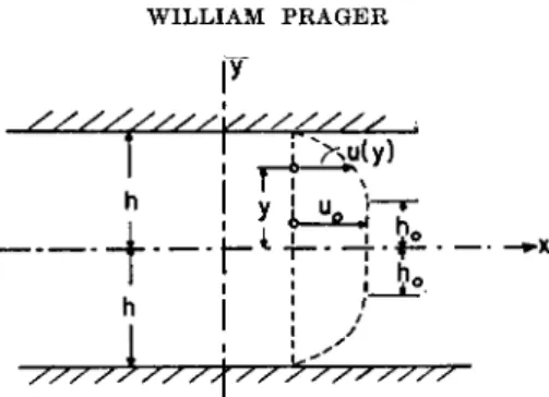
and Hodge.³ FIG. 6. Velocity profile.

The simple shear flow described by (25) and

v = 0 already exhibits an important characteristic of plane plastic flows.

While the velocity profile u{y) must be continuous, the derivative du/dy need not be continuous. For instance, the velocity profile A BCD in Fig. 6 is compatible with the uniform state of stress described by px = py = p, pxy = k: the material below y = 0 remains at rest, and the material above y = h performs a translation normal to the y-axis with the speed U, while the material in the layer 0 < y < h is subjected to simple shear.

Since the material is inviscid, there is no restriction on the intensity of the shear rate U/h. We may therefore consider a sequence of such flow pat- terns for which the value of U remains the same while h tends toward zero. In the limit, a discontinuous velocity field is obtained. If the dis- continuity surface moves with the material, such a field involves rup- ture, a phenomenon that is clearly beyond the scope of the equations of plane plastic flow. While such discontinuous velocity field is there- fore not to be regarded as a physically acceptable solution of these equations, it is a convenient mathematical idealization of a physically acceptable solution with a narrow layer across which the velocity varies rapidly though in a continuous manner. The necessity of justifying dis- continuous flow patterns as mathematical idealizations of physically possible continuous patterns has been ignored in Thomas'¹⁴ recent in- vestigation of surfaces of discontinuity in three-dimensional plastic flow.

The discontinuous shear flow discussed in connection with Fig. 6 is found to share the following properties with all discontinuous fields of plane plastic flow. Firstly, the line of discontinuity is a shear line, i.e., its tangent and normal at a generic point indicate the directions of maximum shearing stress at this point. Secondly, the discontinuity affects only the velocity component in the direction of the tangent to the line of discontinuity; the normal velocity component is continuous. Finally, the jump in the tan- gential velocity component has the same value at all points of the line of discontinuity.

I t can be shown that in a plastic-rigid solid any line separating a region

13 L. Prandtl, Z. angew. Math. Mech. 3, 401 (1923).

14 T. Y. Thomas, J. Rat. Mech. Analysis 2, 339 (1953).

of plastic flow from a rigid region must be a shear line. In many cases the line indicating the plastic-rigid interface will be a line of discontinuity.

6. EXAMPLES OF PLANE PLASTIC FLOW

a. Necking in Tension

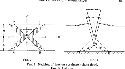
Some of the simplest examples of plane plastic flow involve flow fields that consist of rigid regions separated by lines of discontinuity. Consider, for instance, the infinite solid bounded by the planes y = ± a (Fig. 7), and assume that this solid is subjected to the uniform state of stress speci- fied by px = 2fc, py = 0, pz = k, pxy = pyz = pzx = 0. The components of the stress deviation, found from (3) and (5), are px = k,py = — k, pz = 0, Pxy = Pyz = Ρζχ = 0. The vanishing of pz, pyz, and pzx indicates that we have a problem of plane flow with the x}y plane as the plane of flow. The considered uniform state of stress satisfies the equations of equilibrium (22) and the yield condition (23). The continuous flow field

u — ex v = —cy w = 0 (30\

is compatible with this state of stress; equations (30) describe a uniform rate of extension in the ^-direction combined with a uniform rate of con- traction of equal intensity in the ^/-direction.

An alternative flow field is shown in Fig. 7. The lines AC and BD are lines of discontinuity; they divide the specimen into four parts that move instantaneously as rigid bodies with the same speed in the direction indi- cated by the arrows in Fig. 7. If this discontinuous velocity field is main- tained for a finite period of time, the specimen assumes a shape such as is indicated by the dashed lines in Fig. 7. The discontinuous velocity field does not lead to discontinuous displacements because the particles flow across the stationary surfaces of discontinuity. At the deformed stage under consideration, only the particles in the shaded regions of Fig. 7 have experienced plastic deformation; the other portions of the specimen have moved as rigid bodies.

Obviously, other flow fields are possible under the considered uniform state of stress. For some examples of such fields the reader is referred to Nadai's book.¹⁵ As Onat and Prager¹⁶ have shown, the particular importance of the field of Fig. 7 lies in the fact that it represents the only symmetric solution of the linearized equations of plane plastic flow for a specimen with symmetrically situated, long, and very shallow grooves.

According to Hill,¹⁷ a similar velocity field occurs when a wide metal strip

15 A. Nadai, "Theory of Flow and Fracture of Solids," p. 551. McGraw-Hill, New York, 1950.

16 E. T. Onat and W. Prager, / . Appl. Phys. 25, 491 (1954).

17 R. Hill, J. Mech. Phys. Solids 1, 265 (1953).

F I G . 7. F I G . 8.

FIG. 7. Necking of tension specimen (plane flow).

FIG. 8. Cutting.

is cut in two by means of a tool with a wedge-shaped cutting edge. The tool spans the entire width of the strip which rests on a perfectly smooth, rigid base. The cutting process consists of two phases. During the first, the zones of plastic deformation do not penetrate to the base: on each flank of the tool a "lip" of material is raised as the tool indents the strip (Fig. 8).

This phase will be discussed under c below. Eventually, the horizontal ten- sile stress that is produced in the remaining thickness of material by the penetrating wedge reaches the yield limit, and the second phase begins. The halves of the sheet are now being pushed apart by the wedge; the plastic flow near the upper surface of the strip ceases, and further plastic flow is restricted to two lines of discontinuity (OA and OB in Fig. 8) that pass through the tip of the wedge and intersect the base at 45 deg. In the part of the strip that lies below the tip of the wedge, the velocities relative to the tip correspond to the velocities in the lower half of the tension speci- men in Fig. 7. Corresponding to the "neck" of the specimen, we now ob- serve a small depression at the lower surface of the strip. The dashed lines in Fig. 8 show the strip at such a stage; the full lines indicate the configuration at the beginning of the second phase.

Let us now return to the discussion of the necking of a tension specimen under conditions of plane flow. The velocity field with the lines of discon- tinuity AC and BD in Fig. 7 is compatible with the considered state of stress. This state of stress, however, is possible only in the undeformed specimen but not in the deformed specimen, where it would violate the boundary condition on the sloping parts of the surface. Thus, the velocity field considered is obviously valid at the onset of necking but may lose its validity as soon as some necking has occurred. Before we can accept this velocity field for all stages of the necking process, we must

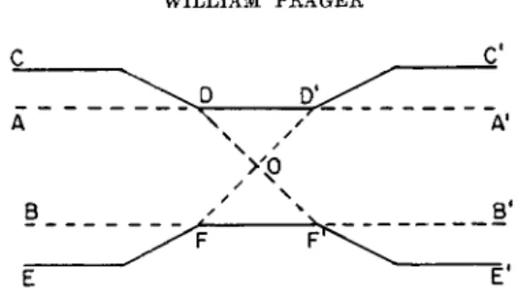
FIG. 9. Discontinuous stress field in necked tension specimen (plane flow).

show that this velocity field is compatible with stresses at or below the yield limit that satisfy the equations of equilibrium and all boundary con- ditions on stress. As Prager¹⁸ has remarked, such a stress field need not be continuous. Indeed, let P be a generic point of a discontinuity surface in the stress field, and choose the x axis normal to the discontinuity surface at P. Equilibrium then requires only that px , pxy , and pzx be continuous;

the other stress components may be discontinuous. Figure 9 shows an equi- librium field of stress that satisfies the boundary conditions on stress and is compatible with the discontinuous velocity field of Fig. 7: the lines A A' and BB' in Fig. 9 represent plane surfaces of discontinuity that are normal to the plane of the figure; the material between these parallel planes is in the state of stress considered above, while the remainder of the specimen is stressfree. The surface portions CD, EF, CD', and E'F' are in the stress- free parts of the specimen and hence free from surface tractions; the surface portions DD^f and FF' are in the stressed part of the specimen but they are free from surface tractions. Thus, the boundary conditions on stress are satisfied over the entire surface of the specimen. Plastic flow is restricted to the planes indicated by the segments DF in Fig. 9, and these segments lie in a region where the stress intensity reaches the yield limit.

Moreover, the considered simple shear along the lines DF is compatible with the state of simple tension that has been assumed between the lines AA' and BB'. We thus have found consistent stress and velocity fields that satisfy all conditions of the theory. We do not claim, of course, that the considered stress field represents the actual stresses in an elastic-plastic specimen, but the existence of this stress field establishes the fact that the discontinuous velocity field discussed in connection with Fig. 7 is acceptable within the framework of the theory of plastic-rigid solids.

b. Sheet Extrusion

The problem of the extrusion of a sheet from the lubricated die shown in Fig. 10 leads to a velocity field that involves circular as well as straight

18 W. Prager, in "Courant Anniversary Volume," p. 289. Interscience Publishers, New York, 1948.

F I G . 10. Sheet extrusion.

lines of discontinuity. For brevity, we will discuss the stress and velocity fields above the axis of symmetry only. The billet moves to the right with the speed V. Plastic flow is restricted to the line AB and the sector OBC;

the lines AB and OC and the arc BC are lines of discontinuity. The ma- terial in the triangle OAB moves as a rigid body with the speed Vy/2 in the direction of the die wall AO. The radial and circumferential velocity components at a generic point in the sector OBC are

u = ^{■ V COS φ} 7(1 + sin φ) (31) Finally, the extruded sheet moves to the right with the speed 7(1 + V2).

It is readily checked that only the tangential velocity component suffers a discontinuity across each line of discontinuity whereas the normal velocity component is continuous. The velocity field therefore is acceptable from the purely kinematical point of view.

Let us now check whether a statically acceptable stress field can be associated with this velocity field. The velocity field within the sector OBC is of the form (29); the corresponding stress field must therefore satisfy (27) and (28). The shear rate Ότφ computed from (31) is

7 _ 1 du dv __ v _ __ 7

jjr __ _ - j - __. _ —

r θφ dr r r (32)

Since this shear rate is negative, the shearing stress γτφ must also be nega-

tive. Equations (27) are therefore valid in the form

Vr = 0 ν'τΨ = ~k (33)

According to the second equation (33), the shearing stress transmitted to the extruded sheet across the line OC is directed from 0 toward C. Now, the sheet is not drawn out of the die but extruded freely. The resultant of all stresses transmitted across OC must therefore be vertical so as to be bal- anced by the resultant of the stresses transmitted across O'C. This condi- tion is fulfilled if the mean normal stress on OC is

p = -k for φ = ΚΤΓ (34)

Since (33) corresponds to the choice of the lower sign in (27), equation (28) must also be used with the lower sign. With the initial condition (34), equation (28) then yields

p = k(2<p - 1 - Υ2π) (35)

in OBC. From (33) and (35) it follows that

pi = 0 pxy=-k p = -fc(l + y2ir) (36) along OB. Throughout the triangle OAB we have the uniform state of stress

specified by (36). Since OA intersects the shear lines OB and AB at 45 deg., OA is a line of principal stress. This means that there is no shearing stress transmitted across OA; the considered stress field can therefore be valid for a lubricated die only.

Before we can accept this stress field, however, we must show that it can be extended into the rigid regions to the left of ABC and the right oi OC in such a manner that the equations of equilibrium and the boundary conditions on stress are satisfied and the stress intensity does nowhere ex- ceed the yield limit. The extension to the right of OC is trivial; the following stresses satisfy all conditions:

Px = 0 py = — 2/c pxy = θ]

in OCD, [ (37) Ρχ = Py = Pxy = 0 J

to the right of OD. Note that the line OD is a line of discontinuity in this extended stress field. The extension of the stress field to the left of ABC is less simple and will not be discussed here. The fact that the stress field can be extended in the desired manner into the billet and the sheet indi- cates that the considered velocity field represents a solution of the prob- lem within the framework of the theory of plastic-rigid solids.

The average extrusion pressure is readily determined. Since no stresses

are transmitted across OD, the extruding force acting on the upper half of the billet must equal the horizontal component of the force transmitted on the die wall 0A; this force, in turn, equals the sum of the horizontal forces transmitted across AB and BO. According to (36), the horizontal stress components are px = p + px = — fc(l + K**) on AB and pxy = p'xy = —k on BO. Since AB = BO = Λ'Λ/2, the required horizontal force is

H = Vi ^k ( ^{2 +} l·) ⁽³⁸⁾

To obtain the average extrusion pressure p, we must divide this force by- one half of the thickness h of the billet. Since h = h!(l + \ / 2 ) , we find

* - * 2 + ^

The stream lines of the flow through the die are readily constructed. To the left of ABC and to the right of OC the streamlines are parallel to the axis of symmetry; in the triangle OAB they are parallel to the die wall AO.

In the sector OBC equations (31) define the angle at which the stream lines intersect a given ray through 0. When this angle is evaluated for a few rays, the stream lines are easily drawn so as to intersect these rays at the proper angles. The lower half of Fig. 10 shows stream lines that have been obtained in this manner.

For a discussion of other extrusion problems the reader is referred to a paper by Hill.¹⁹

c. Wedge Indentation

The sheet extrusion discussed above constitutes a problem of steady flow:

the velocity field does not change with time. The necking process discussed in connection with Figs. 7 and 9 may be described as pseudosteady because the velocity field preserves its character while the slip bands DF' and D'F (Fig. 9) decrease in length. Another problem of pseudosteady plastic flow is the wedge indentation treated by Hill, Lee, and Tupper.²⁰ A lubricated rigid wedge is pressed with uniform velocity into a semi-infinite plastic solid so as to produce plane plastic flow. Figure 11 illustrates an arbitrary stage of the indentation process. Since the depth of penetration is the only characteristic length, the shear line pattern will maintain its shape during the indentation process but will increase in scale proportionally to the depth of penetration. In Fig. 11, the stressfree surface OA of the raised lip and the flank OD of the lubricated wedge represent lines of principle

19 R. Hill, J. Iron Steel Inst. (London) 158, 177 (1948).

20 R. Hill, E. H. Lee, S. J. Tupper, Proc. Roy. Soc. (London) A188, 273 (1947).

FIG. 11. Wedge indentation.

stress that are intersected at 45 deg. by the shear lines BO, BA and CO, CD. The isosceles right triangles OAB and OCD are regions of uniform stress, and the stresses in the sector OBC satisfy equations (27) and (28).

The angle a of this sector is found from kinematical considerations as follows.

Take the vertical velocity of the wedge as the unit of velocity, and count the time t from the instant when the wedge first touches the semi-infinite solid. The depth of penetration then equals t. Let E be the point in the plane of Fig. 11 that lies on the intersection of the undisturbed horizontal surface of the indented solid and the vertical plane of symmetry of the wedge, and denote the distance of E from OA by b. From Fig. 11, we find by elementary trigonometry

b = t sin (ß — a) sin ß + cos (ß — a)

cos ß — sin (ß — a) (40) The line AB CD is a line of discontinuity in the velocity field. At the considered instant, the particles below this line are at rest; the particles just above this line must therefore move along this line. From this condition and equations (26) and (29), it follows that the stream lines in the plastic region are parallel to A BCD.

The velocity in the triangle OCD, which is parallel to DC, and the veloc- ity of the wedge must have the same component normal to OD. The velocity in the triangle OCD therefore has the intensity y/2 sin ß. Since the stream lines are parallel lines, the velocity has the constant intensity y/2 sin ß throughout the plastic region OABCD. The rate at which the distance b increases is given by the component of the velocity in OAB that is normal to OA. This rate of increase is therefore sin ß. Since this rate remains con- stant during the indentation process, and since 6 = 0 when t = 0, we have

b = t sin , (41)

Eliminating the ratio b/t from (40) and (41), we find, after some trigono-

metric transformations,

a + cos"

"' ^tan (i -f)]

It is found that this relation yields a unique value of a for any β between 0 and 90 deg.

The pressure on the flank OD of the wedge is found as follows. Along OA, the principal directions of stress are given by OA and the normal to OA.

Since the principal stress normal to OA is zero, the principal stress parallel to OA must have the intensity 2k. Moreover, this stress must be compres- sive. The mean normal stress in the region of uniform stress OAB has there- fore the value

V = -k (43) The direction of the shearing stress at the line of discontinuity BC must

correspond to the direction of the shearing motion. Thus, the rigid material below BC transmits to the material above BC a shearing stress that is di- rected from B toward C. If the angle φ in the sector OBC is measured in the sense from B toward C so that φ = 0 on OB and φ = a: on OC, the upper sign in equation (27) will be valid in the sector OBC. Accordingly, the upper sign must be taken in equation (28). This equation and the initial condition (43) then furnish p = — fc(l + 2φ) in OBC. In particular,

p = -k(l + 2a) (44) on OC and also throughout the region of uniform stress OCD. In this region,

the principal directions of stress are parallel and normal to OD, and the principal stress parallel to OD must exceed the principal stress normal to OD by 2k if the yield condition is to be satisfied and the shearing stress transmitted across CD is to have the same sense as the shearing motion at this line of discontinuity. Since equation (44) gives the mean of these principal stresses, the stress normal to OD equals — 2fc(l + a). From this and the length OD the vertical force necessary to drive the wedge into the plastic solid is readily determined. Per unit width of the wedge, this force is found to be

F = 4fci(l + a) ^{S i n} ^ T (45)

cos β — sin (β — a)

where a must be determined from the wedge angle β by means of equation (42).

The stream lines and paths of particles coincide in steady flow but not in pseudosteady flow. The path of a given particle is therefore more difficult to trace in pseudosteady flow than in steady flow. A discussion of the tech-

nique of the unit diagram that Hill, Lee, and Tupper²⁰ developed for this purpose would exceed the scope of this article. The left-hand half of Fig. 11 shows the distortion of the originally square meshes of a grid as evaluated by these authors. The exact determination of the distorted grid involves a cumbersome numerical integration. Hodge²¹ has given a convenient approxi- mate method to determine the distortion in problems of this type.

The first phase of the cutting process discussed in connection with Fig. 8 consists of this kind of wedge indentation. The second phase has been treated under a above; it begins when the wedge has penetrated to such a depth that the horizontal stress produced in the remaining thickness of material reaches the yield limit. This depth of penetration depends on the wedge angle and the thickness of the sheet. For a wedge angle 2ß = 20 deg., for instance, the second phase begins when the wedge has penetrated to 45.3% of the sheet thickness (see Hill¹⁷).

The shear line pattern of Fig. 11 has been used by Hill²² to discuss the squashing of a wedge by a lubricated rigid plate and by Lee²³ to discuss the necking of a deeply notched tension specimen.

d. Bulge Test

As has been shown in Section 5, any solution to a problem of plane flow that is acceptable under the yield condition and flow rule of v. Mises is also acceptable under Tresca's yield condition and the associated flow rule.

Since all preceding examples involve plane plastic flow, they do not shed any light on the difference between the two theories. To illustrate this difference, consider the bulge test which is used to determine the ductility of sheet metal under balanced biaxial tension. A circular sheet of uniform thickness is clamped round the periphery and subjected to unilateral fluid pressure, which causes the sheet to bulge plastically. The dimensions of the sheet are chosen so that its flexural stiffness is negligible.

The first consistent theory of the bulge test was given by Hill.²⁴ This theory is based on the yield condition and flow rule of v. Mises; it is approxi- mate because the relevant quantities are represented as power series in the ratio between the maximum deflection and the radius of the die aperture, and powers higher than the second are neglected in the analysis. Hill's theory is therefore restricted to moderate deflections. An alternative theory based on Tresca's yield condition and the associated flow rule has been given by Ross and Prager.²⁵ This theory has the advantage that its equa-

21 P. G. Hodge, Jr., J. Appl. Mechanics 17, 257 (1950).

22 R. Hill, Proc. 7th Intern. Congr. Appl. Mech., London 1, 365 (1948).

23 E. H. Lee, / . Appl. Mechanics 19, 331 (1952).

24 R. Hill, Phil Mag. [7] 41, 1133 (1950).

26 E. W. Ross, Jr., and W. Prager, Quart. Appl. Math. 12, 86 (1954).

tions can be solved in closed form without the use of special assumptions regarding the magnitude of the deflection.

The middle surface of the bulged sheet is a surface of revolution, and the principal stresses at a generic point of this surface are directed along the parallel circle, the meridian, and the normal. In this order, the principal stresses will be denoted by p^c ,p^m , and pⁿ . the initial thickness of the sheet will be denoted by h⁰ and the radius of the die aperture by a. For the usual small values of ho/a, the stress pⁿ is much smaller than the stresses p^c and p^m ; the state of stress at any point of the sheet is therefore essentially one of biaxial tension with the principal stresses p^c and p^m . The sheet material will be treated as plastic-rigid, and the principal rates of extension will be denoted by D^c, D^m , and Dⁿ .

At first glance, one is tempted to assume that the bulge is spherical.

It is easily shown, however, that this assumption is not acceptable under the Mises theory. Indeed, the equations of membrane equilibrium for a spherical bulge require that p^c = p^m . With this state of balanced biaxial tension the flow rule of v. Mises associates strain rates D^c and D^m , which are equal to each other. At the fixed edge of the sheet, however, D^c = 0 whereas D^m > 0.

The considered state of balanced biaxial tension is represented in stress space by a point on an edge of the Tresca prism. Accordingly, the flow rule associated with Tresca's yield condition imposes only one condition on the strain rates D^c and D^m : the rate of dissipation of energy δ = ^i(pcD^c + pmDm) = ^xApJJ>c + D^m) cannot be negative, i.e., D^c + Dm ^ 0 since pc > 0. Thus, the edge conditions, D^c = 0, D^m > 0, do not exclude a spherical bulge if this flow rule is adopted. It is on account of this fact that the analysis of the bulge test is considerably simplified when the yield con- dition and flow rule of v. Mises is replaced by Tresca's yield condition and the associated flow rule. For the details of this analysis, we refer the reader to the paper by Ross and Prager.²⁵ We mention here only that the considered spherical bulge of uniform wall thickness found to become un- stable λνηβη the wall thickness has been reduced to % of the original thick- ness of the sheet.

III. Flow of Work-Hardening Plastic Solids

The mechanical behavior of a perfectly plastic solid is defined by a rela- tion between the instantaneous strain rate and stress, and this relation is independent of any plastic deformations that may have occurred prior to the considered instant. The strain with respect to a fixed reference state thus does not enter into the fundamental equations of the theory of per- fectly plastic solids, and the mathematical difficulties inherent in the con-