Complete dispersion characterization of microstructured optical fibers using windowed Fourier-transform spectral interferometry

(1)

PROCEEDINGS OF SPIE

SPIEDigitalLibrary.org/conference-proceedings-of-spie

Complete dispersion characterization of microstructured optical fibers using windowed Fourier-transform spectral interferometry

M. Horváth, T. Grósz, B. G. Nagyillés, K. Vuković, A. P.

Kovács

M. Horváth, T. Grósz, B. G. Nagyillés, K. Vuković, A. P. Kovács, "Complete

dispersion characterization of microstructured optical fibers using windowed

Fourier-transform spectral interferometry," Proc. SPIE 11029, Micro-structured

(2)

Complete dispersion characterization of microstructured optical fibers using windowed Fourier-transform spectral interferometry

M. Horváth,

^a,b,*

T. Grósz,

^a,c

B. G. Nagyillés,

^a

K. Vuković,

^a

A. P. Kovács,

^a,b

a

Department of Optics and Quantum Electronics, University of Szeged, Dóm tér 9, H-6720 Szeged, Hungary;

b

Department of Photonics and Laser Research, Interdisciplinary Excellence Centre, University of Szeged, Dóm tér 9, H-6720 Szeged, Hungary;

c

ELI-ALPS, ELI-HU Non-Profit Ltd., Dugonics tér 13, H-6720 Szeged, Hungary

ABSTRACT

Dispersion measurements on a birefringent hollow-core (HC-800-02) and a solid-core (LMA-PM-5) photonic crystal fiber (PCF) are presented using a windowed Fourier-transform (WFT) spectral interferometric method. We investigate the optimal value of the spectral window function of the WFT method to reach the highest accuracy in the dispersion measurement. This requires the knowledge of the precise position of the polarization axes of the fibers. In order to determine the position of the polarization axes we have developed a method based on analyzing the WFT signals, which were obtained from a series of interferograms at different excitation ratios of the polarization modes of the PCFs.

Keywords: photonic crystal fiber, spectral interferometry, dispersion measurement, angular alignment, polarization

1. INTRODUCTION

Photonic crystal fibers (PCFs) are special types of optical waveguides whose structure can be modified almost arbitrarily, therefore the requirements of any specific application, e.g. high-power and low-loss pulse delivery can be met with proper design [1-6]. However, the structure of the manufactured PCFs can be different from the designed geometry, which may cause changes in their optical properties including the dispersion. Therefore, it is important to measure the dispersion of the PCFs as accurately as possible after the manufacturing process. In the case of birefringent fibers the chromatic dispersion belonging to the fast and slow polarization axes of the fiber can be quite different [2,7]. Furthermore, the accuracy of the dispersion measurement is highly dependent on the precise excitation of the polarization modes. Since in birefringent fibers the polarization mode dispersion (PMD) can also be an issue, determining the differential group delay (DGD), i.e. the delay between the orthogonally propagating modes, is also of great importance.

Spectral interferometry is a frequently used method for measuring the chromatic dispersion of optical fibers [8]. The advantage of this method is that it does not require long fiber samples. Several algorithms have been developed to extract the spectral phase from the spectral interferograms [9]. One of them is the Fourier-transform method, which proved to be an accurate evaluation technique for PCFs [7,9,10]. However, if two pulses travel through the fiber, e.g. because both polarization modes are excited, signals belonging to the modes/pulses might overlap in the time domain causing difficulties during the evaluation. It has been demonstrated recently that the chromatic dispersion of PCFs can be retrieved for both polarization axes simultaneously from a single interferogram using the windowed Fourier-transform (WFT) method even when the polarization modes overlap in time [11]. In that case a ridge-based (windowed Fourier-ridges, WFR) algorithm was used during the evaluation of the spectral interferogram. Different angular alignment techniques have been reported with special experimental requirements to determine the position of the polarization axes in birefringent fibers. These techniques either require heating [12] or, mechanical rotation of the fiber [13] or the modulation of the laser frequency [14].

* horvathmercedesz@titan.physx.u-szeged.hu

(3)

In this work, we investigate what the optimal value of the spectral window function of the WFT method is to reach the highest accuracy in the dispersion measurement when the polarization modes of PCFs are excited separately or simultaneously. Furthermore, a WFT-based angular alignment technique is reported, which can be connected to the dispersion measurement of the PCFs without any specific experimental requirements.

2. THEORY

2.1 Spectrally resolved interferometry

Spectrally resolved interferometry requires a two-beam interferometer, a broadband light source and a spectrometer.

The examined optical sample is placed in one arm of the interferometer while the other is used as a reference that produces adjustable delay between the two arms. At certain τ time delays spectral interference fringes appear at the output of the spectrometer. The frequency-dependent intensity distribution of the interference fringes I(ω) can be described with the following expression:

I( ) I_ref( ) I_sam( ) 2  I_ref( ) I_sam( ) cos( ( )),   (1) where Isam(ω) and Iref(ω) denote the spectral intensity distributions of the sample and the reference beams, respectively.

ϕ(ω) is the spectral phase difference between the two arms:

( ) ( ) ,

     (2)

where φ(ω) is the spectral phase of the sample and ωτ is the phase term that depends on the path length difference between the two arms. In most cases the effect of an optical medium on the temporal shape of an ultrashort laser pulse can be characterized by the spectral phase. The coefficients of the Taylor expansion of φ(ω) can be used to describe the spectral phase,

2 3

0 0 0 0 0 0 0

1 1

( ) ( ) ( )( ) ( )( ) ( )( ) ...,

2 6

GD GDD TOD

                 (3) where ω0 is the carrier angular frequency of the pulse. The derivatives of the spectral phase with respect to the angular frequency evaluated at ω0are called the constant phase term (φ(ω0)), the group delay (GD), the group-delay dispersion (GDD) and the third-order dispersion (TOD), respectively, as follows:

0 0 0

2 3

0 0 2 0 3

( ) d , ( ) d , ( ) d .

GD GDD TOD

d _{ } d _{ } d _{ }

  

  

 _  _  _

   (4)

Using these dispersion coefficients, the GDD(ω) function and the dispersion parameter D(ω) of the sample can be calculated as

0 0 0

( ) ( ) ( )( ) ...,

GDD GDD TOD    (5)

2

( ) 2

( ) GDD c,

D L

 

 

   (6)

where λ is the wavelength, c is the velocity of light in vacuum, and L stands for the length of the optical medium, e.g. fiber.

2.2 Windowed Fourier-transform evaluation method

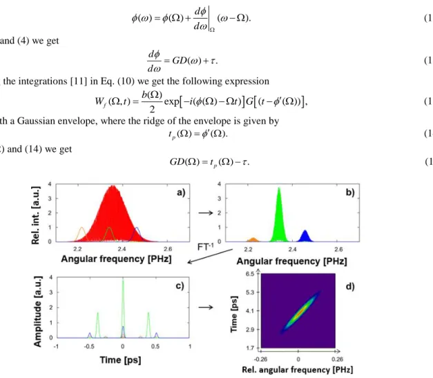
There are several methods for the evaluation of the recorded spectral interferograms and to retrieve the spectral phase and thus the dispersion of an optical sample [9]. In this work the windowed Fourier-ridges algorithm was used to evaluate the interferograms. The steps of the evaluation method are illustrated in Fig. 1. First, an inverse Fourier-transform is performed on the intensity distribution of the interferogram given by Eq. (1) that is multiplied by a window function [Fig.

1(a)]:

( , ) ( ) ( ) exp( ) ,

WI t ^I  g  i t d 



 



  ⁽⁷⁾

where

2

( ) exp

g      ⁽⁸⁾

(4)

is a Gaussian window function, Ω is the central angular frequency and ΔΩ is the width of the window function. A series of windowed interferograms is obtained by changing Ω [Fig. 1(b)]. Introducing a

 

 Isam

 

 Iref

 

 and

 

² sam

   

ref

b   I  I  , and exchanging the cosine function in Eq. (1) with the corresponding complex exponential function we get

( ) ( )

( ) ( ) exp( ( )) exp( ( )).

2 2

b b

I  a   i    i  (9)

Since a(ω) in Eq. (9) is a slowly varying function of ω its inverse Fourier-transform appears around t = 0. On the other hand, b(ω), which contains the important information on the dispersion of the sample, changes rapidly with ω and its inverse Fourier-transform results in two symmetrical signals around τ+GD(ω0) and –τ– GD(ω0) [Fig. 1(b)]. Considering the one appearing at τ+GD(ω0) from Eq. (7) we get

 

( , ) ( ) ( ) exp ( ) .

f 2

W t ^ b g  i t i  d



 



   ⁽¹⁰⁾

The width ΔΩ of the spectral window function should be set to meet the following two requirements: in the vicinity of Ω the fringe amplitude should be constant, i.e., b(ω) = b(Ω) and the spectral phase can be approximated by a linear function, i.e.,

( ) ( ) d ( ).

d

    

_

     (11)

From Eqs. (2) and (4) we get

( ) .

d GD

d

  

 ^ ^ ⁽¹²⁾

By performing the integrations [11] in Eq. (10) we get the following expression

   

( , ) ( )exp ( ( ) ) ( ( )) ,

f 2

W t b^ i   t G t (13) i.e. a signal with a Gaussian envelope, where the ridge of the envelope is given by

( ) ( ).

tp   (14)

Using Eqs. (12) and (14) we get

( ) _p( ) .

GD t   (15)

Fig. 1. Steps of the windowed Fourier-transform method: (a) the intensity distribution of the interferogram multiplied by Gaussian window functions, (b) series of windowed interferograms by changing the central angular frequency of the window function, (c) symmetrical signals after performing an inverse Fourier-transform on the interferograms and (d) the resulting WFT signal.

(5)

By determining the ridges of the WFT signal, tp at each Ω frequency the relative GD curve of the sample can be obtained [Fig. 1(d)]. If the time delay τ is changed, the relative GD curve moves along the time axis, but since its shape does not change the relative GD of the sample can be determined by fitting a polynomial to the ridges. Differentiating Eq. (15) the GDD of the sample can also be retrieved

( ) dt^p. GDD  d

 ⁽¹⁶⁾

Using Eq. (6) the dispersion parameter of the sample can be evaluated:

2

( ) 2 cdt^p.

D Ld



  

 ⁽¹⁷⁾

Although D is not dependent on the time delay τ, selecting the proper delay is of crucial importance since it is proportional to the fringe density and thus affects the visibility.

Consider the case when two pulses having orthogonal polarization directions propagate in the sample arm. Eq. (1) is modified as

( ) ( ) ( ) ( ) 2 ( ) ( ) cos( ( ))

2 ( ) ( ) cos( ( )) 2 ( ) ( ) cos( ( )),

ref samX samY ref samX X

ref samY Y samX samY XY

I I I I I I

I I I I

       

       

    

  ⁽¹⁸⁾

where I_samX I_samX₀cos²and I_samY I_samY₀sin²are the projections of intensities of the sample pulses onto the plane of the polarization of the reference pulse. α denotes the angle between the polarization plane x-z of the sample pulse and the polarization plane of the reference pulse. I_samX₀ and I_samY₀ are the intensities of the sample pulses polarized linearly in the x-z and y-z planes, respectively. The first two interference terms express the interference of the reference pulse and the sample pulse propagating along the fast (X) and the slow (Y) axes, respectively, and the last term describes the interference between the sample pulses. The corresponding spectral phases can be written as

( ) ( ) ,

( ) ( ) ( ).

X X

Y Y

XY X Y

    

     

 

 

(19) In this case the W_f( , ) t is composed of three terms, thus three tp can be defined:

( ) ( ),

( ) ( ).

pX X

pY Y

pXY XY

t t t



   

(20)

Note, that the interference of the two sample pulses with each other and the reference pulse results in three GD curves:

( ) ( ) ,

( ) ( ).

X pX

Y pY

pXY

GD t

DGD t



   

  

(21)

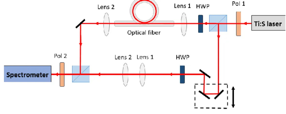
3. RESULTS AND DISCUSSION 3.1 Experimental setup

The experimental setup as shown in Fig. 2 was based on a Mach-Zehnder interferometer illuminated by a Ti:Sapphire laser (Femtolasers, Rainbow, producing pulses of 6 fs at 800 nm, FWHM = 150 nm). The samples, an 89.9-cm-long, hollow-core (HC-800-02, NKT Photonics) and a 92.5-cm-long, solid-core (LMA-PM-5 PCF, NKT Photonics) fiber, were placed into the sample arm and a high-resolution spectrometer (Ocean Optics, HR4000, 700 to 900 nm, spectral resolution 0.2 nm) was placed at the output of the interferometer. Both optical fibers were birefringent. A half-wave plate (HWP) was placed in the sample arm before the fibers to adjust the excitation of the polarization modes of the fibers. Another half- wave plate was put in the reference arm to produce beams with matching polarization. A polarizer (Pol 1) was put before the input of the interferometer to ensure the purity of the linear polarization. The light was coupled into the fibers with a

(6)

30.0-mm-focal-length NIR achromatic lens (Lens 1) and a 19.0-mm-focal-length NIR achromatic lens (Lens 2) was placed after the fibers as collimating optics. The same lenses were placed in the reference arm to compensate their dispersion in the sample arm. A polarizer (Pol 2) at the output of the interferometer was used to optimize the visibility of the interference fringes and to facilitate the interference of orthogonally polarized beams if set to 45° with respect to the interfering polarization directions.

Fig. 2. Experimental setup: spectrally resolved Mach-Zehnder interferometer with the studied fibers in the sample arm.

Measurements were performed under different excitation conditions of the tested fibers. In the first case the fast or the slow polarization mode was excited separately and interfered with the reference beam. In the second measurement both polarization modes were excited simultaneously and interfered with each other and also with the reference beam.

Interferograms were recorded at different τ time delays between the two arms in both aforementioned cases. When both polarization modes were excited simultaneously without the reference beam, a PMD measurement was performed.

3.2 Optimal value of the width of the spectral window function

First, we investigated the optimal width of the spectral window function of the windowed Fourier-transform method to reach the highest accuracy in the dispersion measurement. By reducing the width of the window function the spectral resolution is improved and the requirement in Eq. (11) is also met. However, it results in a worse temporal resolution of the signal, because

8 ln(2) tFWHM 

  , ⁽²²⁾

where t_FWHM is the full width of half maximum of the pulse. Increasing the width of the window the temporal resolution becomes better, however, the linear approximation of the spectral phase is not fulfilled at a certain width of the window function. Due to the effect of the second order the pulse is broadened in time but the maximum of the pulse is not shifted.

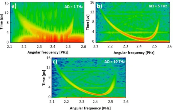
However, the third order causes asymmetry in the shape of the pulse, which shifts the maximum of the pulse, therefore its effect must be eliminated. Considering these, the optimal value of the width of the window function was selected to reach a balance between the temporal and the spectral resolution of the WFT signal. The investigation was based on empirical facts in the case of both fibers. As an example, the resulting WFT signals of the fast mode excited in the hollow-core fiber are shown in Fig. 3. When setting ΔΩ at 1 THz neither the temporal nor the spectral resolution was high enough therefore the WFT signal spread both temporally and spectrally [Fig. 3(a)]. By increasing the width of the window function to 5 THz the temporal shape of the resulting WFT signal became well-defined while the spectral resolution also improved [Fig.

3(b)].

(7)

Fig. 3. WFT signals of the fast polarization mode excited in the hollow-core fiber when the width of the window function is set to (a) 1 THz, (b) 5 THz and (c) 10 THz.

By selecting a 10-THz-wide window function the temporal resolution increased further [Fig. 3(c)], however, even the smaller, 5 THz width was sufficient for precise dispersion measurement under all excitation conditions of the hollow-core fiber. Note that in the case of the solid-core fiber the 5 THz width of the window function was favorable only when the two polarization modes were excited separately but when they were excited simultaneously not even the 10-THz-wide window function was enough (see chapter 3.4).

3.3 Dispersion measurement of the hollow-core fiber

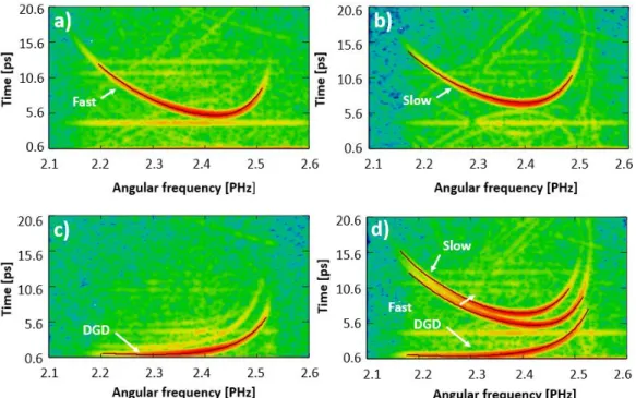
After selecting the optimal width of the window function 10 spectral interferograms were evaluated for all excitation conditions. The resulting WFT signals are shown in Fig. 4. As can be seen, by determining the ridges of the signals the relative GD curves and DGD curve could be retrieved even when both polarization directions were excited simultaneously and interfered with the reference beam. Based on these observations recording a single interferogram is sufficient to retrieve the relative GD curves and thus the dispersion properties of both polarization modes and the DGD curve at the same time.

To confirm this statement, the D curves were determined and compared with each other for the different excitation conditions of the fiber.

(8)

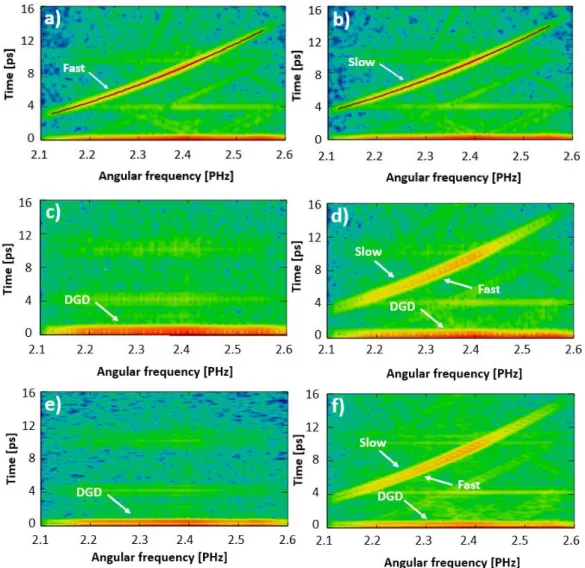
Fig. 4. Windowed Fourier-transform of the recorded interferograms when (a) only the fast or (b) the slow mode interferes with the reference beam individually, when (c) both polarization modes are excited simultaneously without the reference beam, and when (d) both polarization modes are excited simultaneously with the reference beam. These WFT signals were obtained at the same τ time delay between the two arms of the interferometer.

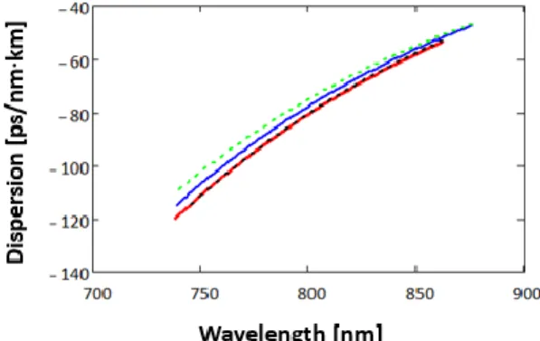
In the evaluation process the best fit to the retrieved relative GD curve was obtained with a seventh-order polynomial, thus the dispersion coefficients for both polarization directions were determined up to the eighth order. The GDD and the D curves were calculated from the dispersion coefficients using Eqs. (5) and (6). The D curves belonging to the fast and the slow polarization axes and the DGD curves were obtained between 752 nm and 858 nm in the case of separate and simultaneous excitation of the two modes, respectively. The resulting curves are shown in Fig. 5.

Fig. 5. (a) Dispersion curves determined during simultaneous excitation of the fast (black curve) and the slow modes (red curve) and separate excitation of the fast (green-dashed curve) and the slow axes (blue-dashed curve). (b) Differential group delay curves normalized to the length of the fiber determined during simultaneous excitation of the polarization modes with (black curve) and without (green-dashed curves) the reference beam.

As can be concluded the curves are completely identical independently from the excitation conditions of the polarization modes. This indeed confirms that a single interferogram is sufficient to the complete dispersion characterization of the tested hollow-core fiber. In addition, the dominance of the higher order dispersion terms can be predicted from the shape of the WFT signals without further analysis.

(9)

3.4 Dispersion measurement of the solid-core fiber

The above mentioned measurements were repeated with a solid-core fiber sample as well, i.e. the spectral interferograms were recorded under all four excitation conditions. First, the width of the Gaussian window function was set to 5 THz. The WFT signals obtained in this case are shown in Fig. 6. As can be seen the ridges of the WFT signals, i.e.

the relative GD curves can be determined for both polarization axes when the fast [Fig. 6(a)] or the slow [Fig. 6(b)] modes were excited separately. However, the temporal resolution was not high enough to determine the ridges of the WFT signals in the case of the PMD measurement or when both polarization modes interfered simultaneously with the reference beam [Fig. 6(c) and (d)]. This can be explained by the very small, about 0.55-ps time delay between the relative GD curves belonging to the fast and the slow modes, which is also observable in Fig. 6(a) and (b). Therefore, the evaluation was performed on the interferograms using a wider, namely a 10-THz window function to increase the temporal resolution of the windowed Fourier-transform. The resulting WFT signals are shown in Fig. 6(e) and (f) without the relative GD curves for the better visibility of the ridges. The WFT signal of the DGD with an almost constant value was well resolved in both cases but the WFT signals of the fast and slow modes still overlapped and could not be separated completely.

Fig. 6. Windowed Fourier-transform of the recorded interferograms obtained with a 5-THz window function when (a) only the fast or (b) the slow mode interferes with the reference beam individually, and when both polarization modes are excited simultaneously (c) without and (d) with the reference beam. WFT signals obtained with a 10-THz window function when (e) both polarization modes are excited simultaneously (e) without and (f) with the reference beam. These WFT signals were obtained at the same τ time delay between the two arms of the interferometer.

(10)

To compare the separated and the simultaneous excitation of the polarization modes the D curves were also calculated in the case of this fiber. The dispersion coefficients were determined up to the third order by a second-order polynomial fitting to the relative GD curve. The D curves were acquired for all excitation conditions from 738 nm to 862 nm and the resulting curves are shown in Fig. 7. As can be seen the D curves were identical when the fast and the slow modes were excited separately using a 5-THz window function. In the case of the simultaneous excitation of the modes the neither the 5, nor the 10-THz width was precise enough. The agreement between the D curves belonging to the two orthogonal polarization axes was expected because of the constant GD difference between them. Consequently, the DGD, obtained by subtracting the GD curves of the two orthogonal modes when they were excited separately had an almost constant value of 0.585 ps/m±0.004 ps/m for the entire wavelength range.

Fig. 7. Dispersion curves along the fast (red curve) and the slow (black dashed curve) polarization directions obtained with 5- THz window function during separated excitation and in the case of simultaneous excitation of the fast (blue curve) and the slow modes (green-dashed curve) obtained with 10-THz window function.

3.5 Measurement of the position of the polarization axes

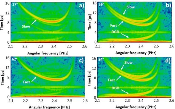
As previously mentioned the windowed Fourier-transform method has a big advantage in contrast to the other evaluation techniques, namely that it provides information on the sign and the dominance of the chromatic dispersion of the fiber. In addition, the intensity of the WFT signals visually provides information on the extent of the excitation of the polarization modes. To prove this hypothesis, we did a measurement by adjusting the angle of the half-wave plate before the optical fiber in one degree steps over the entire 360° range at a given time delay, i.e. the excitation ratio of the two polarization modes. The polarizer at the output of the interferometer and the half-wave plate in the reference arm were set to 45° with respect to the polarization directions of the fiber to get interference in every HWP position. Note that these measurements were feasible only in the case of the hollow-core fiber since the interference of both polarization modes of the solid-core fiber with the reference beam produced indistinguishable WFT signals [recall Fig. 6(d) and (f)].

Four WFT signals obtained by the evaluation of the interferograms are shown in Fig. 8. As can be seen only the WFT signal of the slow mode appeared when the angle of the HWP was set to 17°, i.e. only the slow polarization mode was excited. When the value of the angle was adjusted to 39° the WFT signals of the fast mode and the DGD also appeared along with the one belonging to the slow mode. The WFT signals of the slow mode and the DGD disappeared when the angle of the HWP was adjusted further to 62° thus only the fast polarization mode was excited. At 84° all the three above mentioned signals appeared again. According to these measurements it is possible to determine the angle of the HWP at which the fast or the slow mode is excited the most, i.e. the position of the polarization axes of the fiber can be determined.

This knowledge contributes to precise chromatic dispersion measurement as well.

(11)

Fig. 8. WFT signals under different excitation conditions when the half-wave plate before the fiber was set to the angle of (a) 17°, (b) 39°, (c) 62° and (d) 84°.

The steps of our method are depicted in Fig. 9. The windowed Fourier-transform was performed on the interferograms but only at a selected central angular frequency of the spectral window function, namely at 2.355 PHz corresponding to the 800 nm central wavelength of the Ti:Sapphire laser. This way the WFT signals were obtained only at that frequency as if taking a section from the previous WFT signals [Fig. 9(a)]. As shown in Fig. 9(b) the WFT signals retrieved in such a manner were well separated temporally at the chosen frequency thus the intensity maxima of the signals corresponding to the two polarization modes could be determined. Provided that the evaluation is performed on all 360 interferograms the change in the intensity of the signal belonging to a given polarization axis can be determined depending on the angle of the HWP.

Fig. 9. Determination of the position of the polarization axes: (a) a section of the WFT signals is taken at 2.355 PHz central angular frequency of the window function, (b) the relative intensity of the selected section as a function of the time delay and (c) the relative intensity in the case of the signal belonging to the fast axis as a function of the angle of the half-wave plate.

(12)

The intensity of the fast polarization mode as a function of the angle of the half-wave plate is depicted in Fig. 9(c). A cosine function was fit to the measured data to determine the angle belonging to the most excited state of the mode. The resulting value of the position of the fast axis was 62.49°±0.3°. Naturally, the position of the slow axis can be determined in the same way.

The advantage of the method is that it does not require a specific experimental setup thus it is possible to do this measurement before the dispersion measurement of the fiber. On the other hand, the number of the recorded interferograms is quite high and the method can be used only if the WFT signals of the modes are well separated in the time domain, i.e.

at least 1 ps time delay is needed between the modes.

4. CONCLUSION

The WFR algorithm was applied for dispersion retrieval at a hollow-core (HC800-02) and a solid-core (LMA-PM-5) fiber utilizing a Mach-Zehnder interferometer illuminated by a Ti:Sapphire laser. A high-resolution spectrometer was used during the measurements. The optimal value of the spectral window function was investigated and it was found that the 5- THz-width was sufficient for accurate chromatic dispersion measurement of the fibers when the polarization modes were excited separately. In the case of the hollow-core fiber the DGD curves and the D curves of the fast and the slow polarization modes were obtained between 752 nm and 858 nm, and it was sufficient to record a single interferogram to determine these curves. However, in the case of the solid-core fiber the D curves along the fast and the slow modes could have been retrieved from 738 nm to 862 nm only when the two modes were excited separately. Even though the width of the window function was increased to 10 THz that was not enough to resolve the spectrally and temporally overlapped signals of the two orthogonal modes of the solid-core fiber. The DGD curve had an almost constant value of 0.585 ps/m±0.004 ps/m, which was obtained by subtracting the relative GD curves of the two polarization modes when they were excited separately.

A method was developed to determine the position of the polarization axes of the hollow-core fiber based on the observation of the excitation ratio of the polarization modes. It was shown that the position of the fast polarization axis was at 62.49°±0.3°. This method was not suitable to examine the solid-core fiber because that would have required at least a 1-ps time delay between the two polarization modes.

ACKNOWLEDGEMENT

Supported by the UNKP-18-3 New National Excellence Program of the Ministry of Human Capacities.

The project has been supported by the European Union, co-financed by the European Social Fund. EFOP-3.6.2-16-2017- 00005, “Ultrafast physical processes in atoms, molecules, nanostructures and biological systems“

Ministry of Human Capacities, Hungary grant 20391-3/2018/FEKUSTRAT is acknowledged.

The ELI-ALPS project (GINOP-2.3.6-15-2015-00001) is supported by the European Union and co-financed by the European Regional Development Fund.

REFERENCES

[1] J. Broeng, S. E. Barkou, T. Sondergaard, and A. Bjarklev, “Analysis of air-guiding photonic bandgap fibers,” Opt.

Lett. 25(2), 96–98 (2000).

[2] G. Bouwmans, F. Luan, J. C. Knight, P. St. J. Russell, L. Farr, B. J. Mangan, and H. Sabert, “Properties of a hollow- core photonic bandgap fiber at 850 nm wavelength,” Opt. Express 11(14), 1613–1620 (2003).

[3] W. Göbel, A. Nimmerjahn, and F. Helmchen, “Distortion-free delivery of nanojoule femtosecond pulses from Ti:sapphire laser through a hollow-core photonic crystal fiber,” Opt. Lett. 29(11), 1285–1287 (2004).

[4] A. A. Ishaaya, C. J. Hensley, B. Shim, S. Schrauth, K. W. Koch, and A. L. Gaeta, “Highly-efficient coupling of linearly- and radially-polarized femtosecond pulses in hollow-core photonic band-gap fibers,” Opt. Express 17(21), 18630–18637 (2009).

[5] N.A. Mortensen, M.D. Nielsen, J.R. Folkenberg, A.Petersson, H.R. Simonsen, “Improved large-mode-area endlessly single-modephotonic crystal fibers,” Opt. Lett. 28(6), 393-395 (2003).

[6] B. Zsigri, C. Peucheret, M.D. Nielsen, P. Jeppesen, “Transmission over 5.6 km large effective area and low-loss (1.7 dB/km) photonic crystal fibre,” Electron. Lett. 39(10), 796-798 (2003).

(13)

[7] T. Grósz, A. P. Kovács, and K. Varjú, “Chromatic Dispersion Measurement along Both Polarization Directions of a Birefringent Hollow-core Photonic Crystal Fiber Using Spectral Interferometry,” Appl. Optics 56(19), 5369–5376 (2017).

[8] M. A. Galle, W. Mohammed, L. Qian, and P. W. E. Smith, “Single-arm three-wave interferometer for measuring dispersion of short lengths of fiber,” Opt. Express 15(25), 16896–16908 (2007).

[9] T. Grósz, A. P. Kovács, M. Kiss, and R. Szipőcs, “Measurement of higher order chromatic dispersion in a photonic bandgap fiber: comparative study of spectral interferometric methods,” Appl. Optics 53(9), 1929–1937 (2014).

[10] M. Takeda, H. Ina, and S. Kobayashi, “Fourier-transform method of fringe-pattern analysis for computer-based topography and interferometry,” J. Opt. Soc. Am. 72(1), 156–160 (1982).

[11] T. Grósz, M. Horváth, and A. P. Kovács, “Complete dispersion characterization of microstructured optical fibers from a single interferogram using the windowed Fourier-ridges algorithm,” Opt. Express 25, 28459 (2017).

[12] N. Caponio, C. Svelto, “A Simple Angular Alignment Technique for polarization-maintaining-fiber,” IEEE Photonics Technology Lett. 6(6), 728-729 (1994).

[13] Y.Ida, K. Hayhasi, M. Jinno, T. Horii, K. Arai, “New method for polarization alignment of birefringent fiber with laser diode,” Electron. Lett. 21(1), 18-19 (1985).

[14] D. O. Maionchi, W. Campos, J. Frejlich, “Angular alignment of polarization-maintaining optical fiber.” Opt. Eng.

40(7), 1260-1264 (2001).