Period function of planar turning points

(1)

Period function of planar turning points

Renato Huzak

¹

and David Rojas

^B²

1Hasselt University, Campus Diepenbeek, Agoralaan Gebouw D, 3590 Diepenbeek, Belgium

2Departament d’Informàtica, Matemàtica Aplicada i Estadística, Universitat de Girona, Girona 17003, Catalonia, Spain

Received 17 November 2020, appeared 22 March 2021 Communicated by Armengol Gasull

Abstract.This paper is devoted to the study of the period function of planar generic and non-generic turning points. In the generic case (resp. non-generic) a non-degenerate (resp. degenerate) center disappears in the limit e → 0, where e ≥ 0 is the singular perturbation parameter. We show that, for each e >0 and e∼ 0, the period function is monotonously increasing (resp. has exactly one minimum). The result is valid in an e-uniform neighborhood of the turning points. We also solve a part of the conjecture about a uniform upper bound for the number of critical periods inside classical Liénard systems of fixed degree, formulated by De Maesschalck and Dumortier in 2007. We use singular perturbation theory and the family blow-up.

Keywords: critical periods, family blow-up, period function, slow-fast systems.

2020 Mathematics Subject Classification: 34E15, 34E17.

1 Introduction

We consider slow-fast polynomial Liénard equations of center type

Xe,η :











x˙ =y−

x²ⁿ+

∑

l k=1

a_kx²ⁿ⁺^2k

,

˙ y=e²ⁿ

−x²ⁿ⁻¹+

∑

m k=1

b_kx²ⁿ⁺^2k⁻¹

,

(1.1)

where l,m,n ≥ 1, η := (_a₁_{, . . . ,}_a_l_,_b₁_{, . . . ,}_b_m)is kept in a compact set K of R^l⁺^m ande≥ 0 is the singular perturbation parameter kept small. SystemX_e,η is invariant under the symmetry (x,t) → (−x,−t) and has a center at the origin for all e > 0, e ∼ 0, and for all η ∈ K.

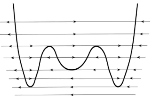
The center is non-degenerate when n = 1 or nilpotent when n > 1. In the limit e = 0, we encounter drastic changes in the dynamics of (1.1): the system has a curve of singular points, given by {y= x²ⁿ+_∑^l_k₌₁a_kx²ⁿ⁺^2k}, passing through the origin, and horizontal regular orbits (see Figure1.1).

BCorresponding author. Email: david.rojas@udg.edu

(2)

Figure 1.1: Dynamics ofX_0,η with 5 contact points.

A portion of the curve of singularities near the origin consists of the normally attracting part{x>0}, the normally repelling part{x <0}and the contact point(x,y) = (0, 0)between them. We call the contact point a turning point because closed orbits surrounding the center, fore>0 small, pass from the attracting part to the repelling part of the curve of singularities.

Whenn=1, the turning point at the origin is generic (sometimes called simple). Whenn>1, we deal with a non-generic or degenerate turning point.

The period function of a center assigns to each periodic orbit its minimal period. Isolated critical points of the period function are called critical periods (or critical periodic orbits) and are central in the qualitative study of the period function. One can note that critical periods do not depend on the parametrization of the set of periodic orbits used. Indeed, if {γ_s}_s_∈(_0,1₎ is such a parametrization ands 7→ T(s)is the period of the periodic orbit γ_s, for any diffeomorphism s 7→ ξ = ξ(s), _ds^dT(ξ(s)) = _dξ^dT(ξ(s))_ds^dξ(s). Therefore the number of isolated zeros of _ds^d(T◦ξ)and _ds^dT are the same.

The main purpose of this paper is to give a complete local study of the period function of X_e,η, near the center at the origin, in both the generic and non-generic case. The study is valid in a small fixed neighborhood of the turning point that is independent of (e,η). Thus, the neighborhood does not shrink to the origin ase→0. In the generic (resp. non-generic) case, the period function of the center in X_e,η is strictly monotonous increasing (resp. has exactly one critical period which is a minimum). More precisely, let us denote byT(y;e)the period function of the center at the origin of system (1.1) with e > 0, e ∼ 0, parametrized by the positivey-axis. Then we have:

Theorem 1.1. Let l,m≥₁and n=₁(resp. n>1) be fixed. For any compact K⊂ _R^l⁺^m there exist e₀ >0and y₀ >0small enough such that the period function T(y;e)of the center of system(1.1)is strictly monotonous increasing (resp. has a global minimum) in the interval]0,y₀], for all e ∈]0,e₀] andη∈K.

We prove Theorem1.1in Section3.4. To prove Theorem1.1, we use a blow-up at the origin in the (x,y,e)-space to desingularize system (1.1). Roughly speaking, after the blow-up we distinguish between “very small”, “small” and “intermediate” closed orbits surrounding the center(x,y) = (_{0, 0}). The period function of the center of system (1.1) cannot be studied uniformly in these three regions and we have to use different techniques for each type of closed orbits. To treat the period function near the very small closed orbits (the ones closest to the center), we use Chicone and Jacobs [2], in the generic case, and generalized polar coordinates, in the non-generic case. The small closed orbits can be treated using the monotonicity criterion due to Schaaf [11], in the generic case, and a result due to Sabatini [10], in the non-generic case. The size of the very small and small closed orbits tends to zero ase → 0. In order to

(3)

obtain the result in an(e,η)-uniform neighborhood of(x,y) = (0, 0), the period function near the passage from the small closed orbits to large closed orbits of sizeO(1)in the(x,y)-space has to be studied. In this passage, we encounter the so-called intermediate closed orbits. The period function near such intermediate closed orbits, in both the generic and non-generic case, will be studied using techniques from [6,8], where small-amplitude limit cycles in an e-uniform neighborhood of slow-fast Hopf points have been investigated (the slow-fast Hopf points correspond to the generic case). For more details we refer to Section2.

We point out that Theorem 1.1 can be proved in a more general framework of smooth Liénard systems. More precisely, the same local result is true if we replace (1.1) with {x˙ = y−x²ⁿ+O(x²ⁿ⁺²), ˙y=e²ⁿ −x²ⁿ⁻¹+O(x²ⁿ⁺¹)}whereO(x²ⁿ⁺²)(resp.O(x²ⁿ⁺¹)) is an even (resp. odd)C^∞-perturbation term that may depend on parameters kept in a compact set. The proof in this more general setting is analogous to the proof for polynomial Liénard equations presented in this paper.

Theorem 1.1, in the generic case n = 1, can be used to solve a part of the following conjecture formulated in [4]: there exists a uniform upper bound on the number of critical periods of classical Liénard equations{x˙ =y−G(x), ˙y= −x}whereGis an even polynomial of degree 2N, N≥1, and G(0) =0. Moreover, this upper bound is conjectured to be 2N−2.

Following Theorem 5 in [4], this can be reduced to the following problem: there exist a small e₀ >0 and an integerM >0 such that the slow-fast system







˙ x= y−

x^2N+

N−1 k

∑

=1

c_2kx^2k

,

˙

y= −ex,

(1.2)

has at most Mcritical periods, for alle∈]0,e₀]and(c2,c₄, . . . ,c₂(N−1))∈_S^N⁻². The following result covers the case where the curve of singularities of (1.2), at level e = 0, has only one contact point, the one at the origin(x,y) = (0, 0).

Theorem 1.2. Let c⁰₂ > 0 be small and fixed and let N ≥ 1 be a fixed integer. Denote by C the set of all values (c₂,c₄, . . . ,c₂₍_N₋₁₎) ∈ _S^N⁻² such that c₂ ≥ c⁰₂ and ^G⁰_x⁽^x⁾ > 0 for all x ∈ _R, where G(x) = x^2N +_∑^N_k₌⁻₁¹c_2kx^2k. For any compact set C, with˜ C˜ ⊂ C, there exists a smalle₀ > 0such that system(1.2)has no critical periods for alle∈]0,e₀]and(c₂,c₄, . . . ,c₂₍_N₋₁₎)∈C.^˜

We prove Theorem1.2in Section3.5. Note that keeping the parameter in a compact set ˜C ensures that the critical curve has no contact points other than the origin. The compact set

C˜ ={(c2,c₄, . . . ,c₂₍_N₋₁₎)∈ _S^N⁻² |c2 ≥c⁰₂andc_i ≥0 fori=4, . . . , 2(N−1)}

is always contained in the set Cdefined in Theorem1.2. When N = 1, Theorem1.2 implies that {x˙ = y−x², ˙y = −ex} has no critical periods for all e ∈]_0,e₀], for some small e₀ > _0.

When N = 2, we have to deal with the slow-fast systems {x˙ = y−x⁴±x², ˙y = −ex}. From Theorem1.2follows that the system with the negative sign in front ofx²has no critical periods.

The system with the positive sign in front ofx²is conjectured to have at most 2 critical periods (see [4]). As explained in [4], it is more difficult to deal with the part of the conjecture when the curve of singularities of (1.2) has more contact points.

When c₂ is uniformly nonzero, Theorem 1.1 in the generic case implies that system (1.2) has no critical periods in an e-uniform neighborhood of the origin in the (x,y)-space. It suffices to notice that the change of coordinates (x,y) →(c₂x,c₂y)transforms (1.2) into (1.1).

See Section3.5.

(4)

2 Blow-up and statement of results

2.1 Family blow-up at the origin in the (x,y,e)-space

To be able to study the period function near the turning point, uniformly in(e,η)with e>0 small, we have to desingularize the system X_e,η near (x,y,e) = (_{0, 0, 0}) using the so-called family blow-up. The family blow-up is the following “singular” coordinate change with n≥1:

Ψ:R⁺×_S²₊→_R³:(r,(x, ¯¯ y, ¯e))7→(x,y,e) = (rx,¯ r²ⁿy,¯ re¯), ¯e≥0.

We define the blown-up vector field as the pullback of X_e,η+0_∂e^∂ divided by r²ⁿ⁻¹: ¯Xη :=

1

r²ⁿ⁻¹Ψ^∗ X_e,η+0_∂e^∂

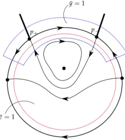
. To study the blown-up vector field ¯X_η (or r²ⁿ⁻¹X¯_η) near the blow-up locus {0} ×_S²₊, it is convenient to use different charts with “rectified” coordinates, instead of the spherical coordinates. For our purposes, only the family chart{e¯ = 1}and the phase directional chart {y¯ = 1} are relevant for the study of the period function since all closed orbits near the center(x,y) = (0, 0)are visible therein (see Figure2.1).

In the family chart{e¯ =1}, we have

(x,y,e) = (rx,¯ r²ⁿy,¯ r)

with (x, ¯¯ y)kept in an arbitrary but fixed compact set. In this chart, r = e and system (1.1) becomesX_F := e²ⁿ⁻¹X¯_F, where

X¯_F :











˙¯

x= y¯−

¯ x²ⁿ+

∑

l k=₁

a_ke^2kx¯²ⁿ⁺^2k

,

˙¯

y= −x¯²ⁿ⁻¹+

∑

m k=1

b_ke^2kx¯²ⁿ⁺^2k⁻¹.

(2.1)

System (2.1) is invariant under the symmetry(x,¯ t)→(−x,¯ −t)and has a center at the origin, for all e ≥ 0, e ∼ 0 andη ∈ K. When e = 0, we are located on the blow-up locus and the vector field (2.1) becomes

(x˙¯=y¯−x¯²ⁿ,

˙¯

y=−x¯²ⁿ⁻¹. (2.2)

A first integral of (2.2) is given by

H(x, ¯¯ y) =e⁻²ⁿ^y^¯

¯

y−x¯²ⁿ+ ¹ 2n

. (2.3)

Note that the invariant curve{y¯= x¯²ⁿ−_2n¹ }is the boundary of the period annulus (see Figure 2.1). The main advantage of the family blow-up is that the blown-up vector field (2.1) has no curves of singularities.

The (x, ¯¯ y)-compact sets in which we will study system (2.1) (see Section2.2) shrink to the origin in the (x,y)-space as e → 0. To obtain (e,η)-uniform results, we also have to study X_e,η in the phase directional chart {y¯ =1}. In the chart{y¯= 1}, we deal with the coordinate change

(x,y,e) = (RX,R²ⁿ,RE)_,

(5)

e¯=1

¯ y=1

p−

p+

Figure 2.1: The family blow-up at the origin (x,y,e) = (0, 0, 0) and dynamics on the blow-up locus. To study the period function of (1.1) in an(e,η)-uniform neighborhood of(x,y) = (0, 0), it suffices to use the charts{e¯=1}and{y¯=1}.

where R ≥ _{0 and} E ≥ 0 are small and X is kept in any compact set. System (1.1) becomes X_D :=R²ⁿ⁻¹X¯_D, where

X¯_D :











X˙ =1−

X²ⁿ+

∑

l k=1

a_kR^2kX²ⁿ⁺^2k

+ ¹

2nXE²ⁿF(X,R,η), R˙ =− ¹

2nRE²ⁿF(X,R,η), E˙ = ¹

2nE²ⁿ⁺¹F(X,R,η),

(2.4)

withF(X,R,η) =X²ⁿ⁻¹−_∑^m_k₌₁b_kR^2kX²ⁿ⁺^2k⁻¹. ForR=E=0, the system has semi-hyperbolic singularities atX=−1 (denoted byp+) andX=1 (denoted byp−). The singularityp+(resp.

p−) has theX-axis as unstable (resp. stable) manifold and a two-dimensional center manifold, transverse to theX-axis.

Using (2.1) and (2.4) we easily detect the singular polycycle Γ on the blow-up locus con- sisting of singularities p+ and p− and the regular orbits that are heteroclinic to them (see Figure2.1). Note that p± are the end points of the regular curve{y¯ =x¯²ⁿ−_2n¹}.

It is clear now that the study of the period function of the center in (1.1), in a small e- uniform neighborhood of (x,y) = (0, 0), can be divided into three parts: the study near the center (x, ¯¯ y) = (0, 0)of (2.1), the study of the interior of the period annulus inside the family (2.1), away from(x, ¯¯ y) = (0, 0)andΓ, and the study nearΓ, combining systems (2.1) and (2.4).

The results related to the first two parts (resp. the third part) are stated in Section 2.2 (resp.

Section2.3).

2.2 Statement of results inside the vector field ¯X_F

Let l,m ≥ 1 be fixed. For the vector field ¯X_F given in (2.1) we define by T_F(y;¯ e)_{the period} function of the center at the origin parametrized by the ¯y-axis. As we will see in Sections3.1 and 3.2, the function T_F(y;¯ e) is well defined in any compact interval [y¯₁, ¯y₂] and when the turning point is generic it can be extended analytically to ¯y =0. We prove the following two

(6)

results concerning the period function of system ¯X_F. The first one states the behaviour of the period function of the center of system (2.1) close to the equilibrium at the origin, whereas the second one is a global statement in the interior of the period annulus.

Theorem 2.1. For any compact K⊂ _R^l⁺^m there existy¯₀> 0small enough and e₀ >0small enough such that _d^d_y_¯TF(y;¯ e)>₀_(resp. _d^d_y_¯_T_F(y;¯ e)<_{0) for n} =₁_{(resp. n}> _{1) for all}y¯ ∈]_{0, ¯}_y₀]_,e∈[_0,e₀] andη∈K. Moreover, T_F(y;¯ e)→2π(resp.+_{∞) as}y¯ →0⁺for n=1(resp. n>1).

Theorem 2.2. For any compact K ⊂ _R^l⁺^m and any 0 < y¯₁ < y¯₂ < +_∞ there existse₀ > ₀small enough such that _d^d_y_¯T_F(y;¯ e)> ₀(resp. _d^d_y_¯²₂T_F(y;¯ e)> 0) for n = ₁(resp. n> 1) for ally¯ ∈ [y¯₁, ¯y₂], e∈ [_0,e₀]andη∈ K.

We prove Theorem 2.1 in Section 3.1 and Theorem 2.2 in Section 3.2. A key fact in the proof of the previous results is that, when e = 0, the vector field (2.1) becomes (2.2) with a first integral given by (2.3). As we will see, the period function of (2.1) is ane-perturbation of the period function of (2.2).

2.3 Statement of results nearΓ

In both the generic and non-generic case, we have the following result about the period function of the center of the vector fieldr²ⁿ⁻¹X¯η, withr>0, in anη-uniform neighborhood of Γ.

Theorem 2.3. Let l,m ≥ 1 be fixed. For any compact K ⊂ _R^l⁺^m there existse₀ > 0 small enough such that the period function of the center of system r²ⁿ⁻¹X¯_η, with r > 0, near the polycycle Γ is monotonous increasing for alle∈]0,e₀]andη∈ K.

We prove Theorem 2.3 in Section3.3. For a precise definition of a neighborhood ofΓ in the family blow-up coordinates and the period function nearΓsee Section3.3.

3 Proof of Theorem 1.1–Theorem 2.3

First we prove Theorem2.1, Theorem 2.2and Theorem2.3. Then we glue them together and prove Theorem1.1(see Section 3.4). Theorem1.2 is proved in Section3.5.

3.1 Proof of Theorem2.1

Let us start considering the casen = 1. We define by T_F(x;¯ e) the period function of system (2.1) parametrized by the ¯x-axis. Notice that, since n = 1, the center at the origin is non- degenerate and therefore the period function can be extended analytically to ¯x =0. Fore≥0 small system (2.1) is an analytic perturbation of the quadratic system

(x˙¯=y¯−x¯²,

˙¯

y=−x.¯ (3.1)

Therefore we can consider the Taylor’s series development ate=0 ofT_F(x;¯ e), T_F(x;¯ e) =T₀(x¯) +O(e),

whereT₀(x¯)is the period function of system (3.1) parametrized by the ¯x-axis. In particular, if

d

dx¯T₀(x¯)>_{0 then} _d^d_x_¯T_F(x;¯ e) >0 for every e≥0 small enough. In consequence, the assertion

(7)

concerning n = 1 in Theorem2.1will follow once we show that the period function T₀(x¯)of the quadratic system (3.1) is monotonous increasing near the origin.

To do so we use Chicone and Jacobs [2] result on quadratic centers to deduce that, in a neighborhood of the origin,

T₀(x¯) =2π+p₂(λ)x¯²+O(x¯³),

where p₂(λ) = ₁₂^π(_16λ²₂ +_8λ₂λ₅+λ²₅+_18λ²₃−_12λ₃λ₆+_9λ₃λ₄+_10λ²₆−λ₄λ₆+λ²₄)_, λ = (λ_i)⁶_i₌₂, andλ_i stand for the coefficients of the Bautin’s normal form for quadratic systems

(x˙ = −y−λ₃x²+ (2λ₂+λ₅)xy+λ₆y²,

˙

y= x+λ₂x²+ (2λ₃+λ₄)xy−λ₂y².

In our case system (3.1) can be brought to the Bautin’s normal form with the change of variable {y¯ 7→ −y¯} and corresponds to the parameters λ₂ = λ₅ = λ₆ = 0, λ₃ = 1 and λ₄=−2. Consequently, for system (3.1) the period function near the origin can be written as

T₀(x¯) =2π+ ^π

3x¯²+O(x¯³).

This fact, together with the discussion at the beginning of the section, shows that there exist e₀, ¯x₀ > 0 small such that _d^d_x_¯T_F(x;¯ e) > 0 for ¯x ∈]0, ¯x₀] ande ∈ [0,e₀]. Since monotonicity is unaltered by parametrization, this finishes the proof of Theorem2.1for the casen=1.

For n > 1 the center at the origin becomes degenerate and Chicone–Jacobs procedure do not apply. With the aim of studying the period function of system (2.1) near the origin (x, ¯¯ y) = (0, 0)forn>1 we consider the change to generalized polar coordinates

(x, ¯¯ y) = (rcosθ,rⁿsinθ) withr ≥0 andθ ∈T. After this change system (2.1) is written as











˙

r= ^r

n

cos²θ+nsin²θ cosθsinθ−_cos²ⁿ⁻¹θsinθ+O(r)_, θ˙= ^r

n−1

cos²θ+nsin²θ

−nsin²θ−cos²ⁿθ+O(r).

We note that terms with e small are inside O(r)so the forthcoming arguments are uniform with respect to e∈ [0,e₀].

For r > 0 small enough we have ˙θ < 0. Therefore we can parametrize the orbits near the origin by ϕ:= −θ. We denote by TF(s;e)the period of the solution r(ϕ,s) and for the sake of simplicity we write f(ϕ) := cos²ϕ+nsin²ϕ, α(ϕ):= cos²ⁿ⁻¹ϕsinϕ−cosϕsinϕ, β(ϕ):= nsin²ϕ+cos²ⁿϕ. Note that β(ϕ) > 0. Due to the symmetry of system (2.1) the functionTF(s;e)writes

TF(s;e) =2 Z ^π

2

−^π₂

dϕ

˙ ϕ =2

Z ^π

2

−^π₂

f(ϕ)dϕ

r(ϕ,s)ⁿ⁻¹ β(ϕ) +O(r(ϕ,s))^. Moreover,

d

dϕr(ϕ,s)

r(ϕ,s) = ^α(ϕ)

β(ϕ)+O(r(ϕ,s)) = ^α(ϕ)

β(ϕ)+O(s),

(8)

where in the second equality we user(ϕ,s) =O(s). Therefore, r(ϕ,s) =r(0,s)e

R_ϕ

0 α(φ) β(φ)+O(s)

dφ= s e

R_ϕ

0 α(φ) β(φ)dφ

+O(s). We denote ρ(ϕ):= e

Rϕ 0

α(φ) β(φ)dφ

> 0. Substituting the previous equality in the expression of TF(s;e)and taking into account thatO(r(_ϕ,s)) =O(s)_{we get}

TF(s;e) = ² sⁿ⁻¹

Z ^π

2

−^π₂

f(ϕ)dϕ

ρ(ϕ) +O(s)ⁿ⁻¹ β(ϕ) +O(s)

= ² sⁿ⁻¹

Z ^π

2

−^π₂

f(ϕ)

ρ(ϕ)ⁿ⁻¹β(ϕ)+O(s)

dϕ

= ² sⁿ⁻¹

_Z π 2

−^π₂

f(ϕ)dϕ

.

Since f,ρandβare positive, the last equality shows thatTF(s;e)→+_∞_ass→₀⁺_forn>_1.

Moreover, d

dsTF(s;e) =−²(n−1) sⁿ

_Z π 2

−^π₂

f(ϕ)dϕ

+ ² sⁿ⁻¹O(1)

= ¹ sⁿ

−2(n−1)

Z ^π

2

−^π₂

f(ϕ)dϕ

.

The last equality shows that _ds^dTF(s;e)→ −_∞ass →0⁺. This ends the proof of Theorem2.1 forn>1.

Remark 3.1. We could also use the following generalized polar coordinates (x, ¯¯ y) = (rρ₁(θ),rⁿρ₂(θ))

where(ρ₁(θ),ρ₂(θ))is the solution of{x˙ =−y, ˙y=x²ⁿ⁻¹}with initial condition(x(0),y(0)) = (1, 0). Using this coordinate change the above expressions become simpler (e.g. β(ϕ) = 1 for allϕ, with ϕ= −θ).

In order to study the global behaviour of the period function of system (2.1) uniformly on e ≥ 0 small in a compact set inside the period annulus it is enough to study the period function of the system (2.2), that is when e = 0. We denote by T₀(y¯) the period function of system (2.2) parametrized by the positive ¯y-axis, and we consider ¯y inside an arbitrary compact interval [y¯₁, ¯y2] with 0 < y¯₁ < y¯2 < +∞. By continuity with respect to the small parametere of system (2.1), taking e small enough the ¯y-axis is also transversal to all orbits of (2.1), which are also periodic for ¯y ∈ [y¯₁, ¯y₂]. We can then define T_F(y;¯ e) as the period function of system (2.1) parametrized by the same ¯yasT0. The function TF(y;¯ e)is analytic for e≥0, e∼0, and so we can consider its Taylor’s series development ate=0,

TF(y;¯ e) =T0(y¯) +O(e).

Then, since the center of system (2.2) is not isochronous, properties of the period function of system for e = 0 are reflected for e ≥ 0 small enough. In particular, _d^d_y_¯T0(y¯) > 0 and

d²

dy¯²T₀(y¯)>0 for all ¯y∈[y¯₁, ¯y₂]will imply _d^d_y_¯T_F(y;¯ e)>0 and _d^d_y_¯²2T_F(y;¯ e)>0 for all ¯y∈[y¯₁, ¯y₂] ande≥0 small, respectively. For this reason, Theorem2.2 is a consequence of the following result.

(9)

Proposition 3.2. The period function of the center(2.2)is strictly monotone increasing for n=1and it is strictly convex for n >1.

The first part of the proof of Proposition 3.2 relies on the application of the following monotonicity criterion due to Schaaf [11].

Theorem 3.3. Consider a Hamiltonian system of the formu˙ =−v,v˙ = g(u), where function g satisfy the following assumptions:

1. g:R→_Ris three times continuously differentiable with g(0) =0and g⁰(0)>0.

2. For all u∈_Rwhere g⁰(u)>0: 5(g⁰⁰)²−3g⁰g⁰⁰⁰

(u)>0.

3. If g⁰(u) =0then g(u)g⁰⁰(u)<0.

Then the origin is a center and the period function is strictly increasing in the whole period annulus.

One of the key elements to prove the second part of Proposition 3.2 is to show that at most one critical period can exist in the interior of the period annulus. To do so we use the following result due to Sabatini [10]. For the sake of shortness in the statement, we define the following operator for smooth functions defined on an interval I:

K[g]:= ^3g

2g⁰⁰²−3gg⁰²g⁰⁰−g²g⁰g⁰⁰⁰

g⁰⁴ .

Theorem 3.4. Consider a Hamiltonian of the form H(u,v) = G(u) +F(v), where G(u) = αu^2k+ o(u^2k) ∈ C^∞(I_G), F(v) = βv²^`+o(v²^`)∈ C^∞(I_F),0 ∈ I_G∩I_F, 0 < k,` ∈ _N, α,β > 0. Here I_G and I_F denote the maximal interval of definition of G and F, respectively. Then the origin is a center and if

µ_s2:=4

1+2GG⁰⁰ G⁰²

FF⁰⁰

F⁰² +K[G] +K[F]

>0 then the period function is strictly convex in the whole period annulus.

Proof of Proposition3.2. The change of variables{u = ln(1+2n(y¯−x¯²ⁿ)),v = x¯} transforms (2.2) into the Hamiltonian system with separable variables

(u˙ =−2nv²ⁿ⁻¹,

˙

v=V_n⁰(u), (3.2)

whereVn(u) = _2n¹ (e^u−u−1). We notice that both periodic functions of system (3.2) and (2.2) are the same through the change of variable. We shall prove the results for (3.2).

Let us prove the first assertion of the statement. To do so, we apply Schaaf’s criterion to system (3.2) with n = 1. After a positive constant rescaling of time and taking g = V₁⁰ we have that the assumptions in Theorem3.3 are fulfilled sinceg⁰(u) =V₁⁰⁰(u) = ¹₂e^u >0 for all u ∈ _R _{and 5}(g⁰⁰)²−3g⁰g⁰⁰⁰

(u) = ¹₂e^2u > _{0 for all} u ∈ R. Therefore the period function of system (3.2) is strictly increasing and so _d^d_y_¯T₀(y¯) > 0 for all ¯y > 0. This proves the assertion concerning n=1.

Let us considern> 1. With the aim of applying Theorem3.4we denote G(u) = V_n(u) =

1

2n(e^u−u−1)and F(v) = v²ⁿ. Clearly the first part of the assumptions of the theorem are fulfilled sinceV_n(u) = _4n¹ u²+o(u²). We claim that µ_s2 ≥ ¹

n² > 0 for alln≥ 2. After showing the inequality, the result follows by direct application of Theorem3.4.

(10)

Using the expressions ofFandGwe have that ˆ

µ_s2(u,n):=µ_s2(u,n)− ¹

n² = ^4e

u

n(e^u−1)⁴^η(u,n),

where η(u,n) = nu²+ (1+3n)u+2n+1+ (2nu²−2u−3n−3)e^u+ ((1−3n)u+3)e^2u+ (n−1)e^3u. A direct computation shows that

d

dnµˆ_s2(u) = ⁴(eû−u−1)eû n²(eû−1)² >0

for allu∈R. Therefore to prove the claim it is enough to show thatη(u, 2)≥0.

We perform a derivation-division procedure with respect to e^u achieving the following equality:

e⁻^u d³ du³

e⁻^u d³

du³η(u, 2)

=216e^u−40u−_156.

The previous expression has exactly two simple negative zeros. Indeed, its derivative is zero only atu = _ln(_5/27), the image at u= 0 is positive and the limits u→ ±_∞_{are both} +_{∞. A} sequence of simple arguments of continuity, number of zeros of the derivative, the values at u = 0 and the values of the limits at ±_∞ yields to show that η(u, 2)≥ 0 for all u ∈ _{R. This} finishes the proof of the claim.

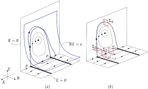
We define a sectionΣ1 ⊂ {X =0}parametrized by (R₁,E₁)∈ [0,R⁰₁]×[0,E₁⁰]for some small R⁰₁,E⁰₁ >0. The sectionΣ1is defined using the coordinates(X,R,E)of (2.4) (we write(R₁,E₁) instead of(R,E) to avoid confusion later). Similarly, we define Σ4 ⊂ {x¯ = 0}parametrized by(y,¯ e), withe∈[0,R⁰₁E⁰₁], where(x, ¯¯ y,e)are the coordinates of (2.1). The sectionsΣ1,Σ4 are transverse to the blown-up vector field ¯X_η and located near the polycycleΓ(see Figure3.1).

Since system (2.1) (resp. (2.4)) is invariant under the symmetry (x,¯ t) → (−x,¯ −t) (resp.

(X,t) → (−X,−t)), it suffices to study the time spent betweenΣ1 andΣ4, i.e. the half time period function of r²ⁿ⁻¹X¯η, denoted by H. Our goal is to prove that LH > 0 on Σ1 (for R⁰₁,E⁰₁ >0 small enough but fixed), withe>0, whereLis the Lie-derivative along the vector field R_∂R^∂ −E_∂E^∂ (see Section 3.3.5). This implies that r²ⁿ⁻¹X¯η (r > 0) has no critical periods nearΓand the period function is monotonous increasing there. Whene=0, system (1.1) has no center.

We aligned up Hin three parts: the timeH_1,2spent betweenΣ1andΣ2(Section3.3.2), the time H2,3 spent between Σ2 and Σ3, near the semi-hyperbolic singularity p− (Section 3.3.1), and the timeH_3,4between Σ3 andΣ4 (Section3.3.3). In Section3.3.4we glue the local results together. Section3.3.5is devoted to the study of the Lie-derivativeLH.

3.3.1 The study ofH_2,3

In this section we study the timeH_2,3inside the familyX_D, i.e. ¯X_D multiplied byR²ⁿ⁻¹. First, we bringXe_D :=F(X,R,η)⁻¹X^¯_D, locally near p− = (_{1, 0, 0}), to a normal form which simplifies the study of H_2,3 (transverse sections Σ2,3 will be defined in the normal form coordinates).

Sincep−is partially hyperbolic for all η∈K, there exists aC^k η-family of center manifolds at p−, given as a graph of X = ₁+ψ(R,E,η) _with ψ(_{0, 0,}η) ≡ 0. Following [5] in the generic

(11)

R=₀

X

R E=0

E

RE=_e

p−

p+

Σ1

Σ2

Σ3

Σ4

(a) (b)

RE=_e

Figure 3.1: (a) Closed orbits near the polycycle Γ, inside RE = e, for a fixed e > _0. _Γ is located on the blow-up locus {r = ₀} (it corresponds to{R = ₀} in the phase directional chart). The center is visible in the family chart. (b) The study of the time spent inside {x ≥ 0} is divided into three parts: Σ1 → _Σ₂, Σ2→_Σ₃ andΣ3→_Σ₄. In the first two parts, we use the vector fieldXD, and in the last part we use X_F.

case or [3] in the non-generic case, an η-family of center manifolds can be chosen to be C^∞ (i.e.ψcan beC^∞). We fix suchψ.

Using the coordinate changeZ=X−(1+ψ(R,E,η)), the fixed family of center manifolds becomes {Z=0}and the vector fieldXeD changes to











Z˙ = − _Φ(R,E,η) +O(Z)Z, R˙ = − ¹

2nRE²ⁿ, E˙ = ¹

2nE²ⁿ⁺¹,

(3.3)

where Φis a smooth function withΦ(0, 0,η) =2n. We used the fact that the family of center manifolds is invariant for Xe_D. Now, we can normally linearize the vector field (3.3) using Theorem 1.1 of [7].

Theorem 3.5. There is a smooth familyΠη :(Z,R,E)→ (Z,^¯ R,E)of local diffeomorphisms, defined in anη-uniform neighborhood of the origin in the(Z,R,E)-space, which brings(3.3)into the normally linearized vector field

Xˆ_D :











Z˙ = −_Φ(R,E,η)Z, R˙ = − ¹

2nRE²ⁿ, E˙ = ¹

2nE²ⁿ⁺¹,

(3.4)

where Φ is defined in (3.3) and where we denote Z again by Z. The diffeomorphisms¯ Πη preserve {RE=const}: Πη(Z,R,E) = (Z(1+Zπ_η(Z,R,E)),R,E)with a smooth familyπ_η.

Remark 3.6. The coordinate change in the normal linearization theorem from [7] isC^∞-smooth and preserves the parameter η and the leaves of the foliation{RE= _const}(the center vari-

(12)

ablesR,Eare preserved). In [6], this normal linearization theorem has been used in the generic case (see also Remark 1.2 in [7]). In the same way we apply it to the non-generic case. We point out that we could also useC^k center manifolds and the normal linearization theorem of [1] with a C^k-coordinate change that preserves η and{RE= const}. The size of the domain of the coordinate change may tend to zero ask →∞. The finite smoothness is not a problem in our proof.

We conclude that, in the normal form coordinates(Z,R,E)of (3.4),X_D can be written as R²ⁿ⁻¹κ(Z,R,E,η)X^ˆ_D, (3.5) whereκ(Z,R,E,η) =F(Z(1+O(Z)) +1+ψ,R,η)andκ(0, 0, 0,η) =1.

In the normal form coordinates, we define Σ2 ⊂ {Z = −Z₀}, parametrized by (R₂,E₂)∈ [0,R⁰₂]×[0,E⁰₂]for some small constants Z₀,R⁰₂,E⁰₂ > 0, andΣ3 ⊂ {E = E₃}, parametrized by (Z,R)_with Z ∼ 0 and R ∈ [_0,R₃]for some small constants R₃,E₃ > 0. All the constants are chosen such that the transverse sectionsΣ2,3 are located in the domain of Π⁻_η¹ and such that the passage w.r.t. ˆX_D betweenΣ2andΣ3 is well-defined.

We can now find the time H_2,3(R₂,E₂) in (3.5), spent between Σ2 and Σ3. Note that the orbit of ˆX_D (or (3.5) with R>0) with the initial point(R₂,E₂)>(0, 0)onΣ2 has the form

Z(E,R₂,E₂)_,^R²^E² E ,E

withZ(E,R2,E2) =−Z0exp −2nRE E2

Φ(^R²_s^E²,s,η) s²ⁿ⁺¹ ds

. Using this, the time H2,3can be written as H_2,3(R₂,E₂) = ²ⁿ

(R₂E₂)²ⁿ⁻¹

Z _E₃

E2

dE

E²κ(Z(E,R₂,E₂),^R²_E^E²,E,η)^. ^(3.6) Since |Z(E,R₂,E₂)| ≤ Z₀ for E ≥ E₂ and κ is positive and bounded for (Z,R,E) ∼ (0, 0, 0) andη∈ K, it is clear that (3.6) tends to+_∞ ase = R₂E₂ → 0, uniformly inη. (Note that the integral in (3.6) is of orderO(_E¹

2).) We will use the expression (3.6) in Section3.3.4.

We conclude this section with a result about the transition map of ˆX_D betweenΣ2andΣ3. Proposition 3.7. There is a C^∞-function J in (R₂,E₂,E²₂lnE₂,η) such that the transition map (R2,E2)→(Z,R)along the trajectories of (3.4)betweenΣ2andΣ3 is given by R= ^R_E²^E²

3 and

Z=−Z0exp

− ¹

E₂²ⁿJ(R2,E2,E²₂lnE2,η)

with J(0, 0, 0,η) =2n.

Proof. When n = 1, the proof of the proposition can be found in [6] (Proposition 4.9). The proof of the case “n>1” is analogous to the proof of the case “n=1”.

Proposition 3.7 implies that the transition map between Σ2 and Σ3 is C^∞-smooth in (R₂,E₂,η). This will be used in the gluing process in Section3.3.4.

(13)

3.3.2 The study of H_1,2

In this section we deal with the timeH_1,2, spent betweenΣ1andΣ2, inside the vector fieldX_D. The smooth sections Σ1,2 are defined above. Note that the system (2.4) has no singularities between Σ1 and Σ2 (since the sectionΣ2 is located uniformly away from the singularity p−, theX-component of (2.4) is strictly positive betweenΣ1andΣ2, for all(R,E)∼(0, 0)and for allηkept in the compact setK). SinceX_D is (2.4), multiplied by R²ⁿ⁻¹, it can be seen that

H_1,2(R₁,E₁) = ¹

R²ⁿ₁ ⁻¹I₁(R₁,E₁,η), (3.7) where I₁is a strictly positiveC^∞-function. We conclude this section with

Proposition 3.8. There exists a C^∞-function J(R₁,E₁,η) such that the transition map(R₁,E₁) → (R₂,E₂)along the trajectories of (2.4)betweenΣ1 andΣ2is given by

(R₂,E₂) =R₁(1+E²ⁿ₁ J(R₁,E₁,η)),E₁(1+E²ⁿ₁ J(R₁,E₁,η))⁻¹.

Proof. In the generic case (n =1), the proof of the proposition is given in [6, Proposition 5.1].

The proof of the non-generic case (n>1) is analogous to the proof of the generic case.

We use (3.7) and Proposition3.8in Section3.3.4.

3.3.3 The study of H_3,4

In this section we deal with the timeH_3,4, spent betweenΣ3andΣ4, inside the vector field X_F (X_Fis equal to (2.1), multiplied by a constante²ⁿ⁻¹= (RE)²ⁿ⁻¹). The smooth sectionsΣ3,4are defined above. If we parametrize Σ3with (x,¯ e)((x, ¯¯ y,e)are the coordinates of (2.1)), then we can write H_3,4 as

H_3,4(x,¯ e) = ¹

e²ⁿ⁻¹I3(x,¯ e,η), (3.8) where I₃ is a strictly positiveC^∞-function. This follows from the fact that the vector field (2.1) is regular along Γon the blow-up locus, betweenΣ3 andΣ4(see Figure3.1).

3.3.4 The study of H

In this section we glue together the local results obtained in Sections 3.3.1–3.3.3and find an expression for the half time period function H. We know that

H(R₁,E₁) =H_1,2(R₁,E₁) +H_2,3(R₂,E₂) +H_3,4(x,¯ e),

where the orbit of r²ⁿ⁻¹X¯η ( ¯Xη is the blown-up vector field defined in Section 2) with the initial point(R₁,E₁)∈_Σ₁intersects sectionΣ2at the point(R₂,E₂)and sectionΣ3at the point (x,¯ e). From (3.6) follows that

H2,3(R2,E2) = ²ⁿ (R₁E₁)²ⁿ⁻¹

Z _E₃

E2

dE

E²κ(Z(E,R₂,E₂),^R¹_E^E¹,E,η)^, ^(3.9) where R₂ and E₂ are the C^∞-functions of (R₁,E₁,η) given in Proposition3.8. Here we used that e= R₁E₁= R₂E₂. Now, we want expressH_3,4(x,¯ e)in terms of(R₁,E₁). Let us recall that the constant E₃ > 0 comes from the definition ofΣ3. Using ¯x = _E^X

3 andX = Z(₁+O(Z)) +

(14)

1+ψ(^R_E¹^E¹

3 ,E₃,η) on Σ3 (O(Z) is a C^∞-function, see Section 3.3.1), and the fact that Z is a C^∞-function in(R₁,E₁,η)(we combine Proposition3.7and Proposition3.8), we see that ¯xis a C^∞-function of(R₁,E₁,η)ande=R₁E₁. This and (3.8) imply that

H_3,4(x,¯ e) = ¹

(R₁E₁)²ⁿ⁻¹^I^˜³(R₁,E₁,η) (3.10) where ˜I₃is a strictly positiveC^∞-function. Combining (3.7), (3.9) and (3.10), we finally get

H(R₁,E₁) = ²ⁿ (R₁E₁)²ⁿ⁻¹

Z _E₃

E2

dE

E²κ(Z(E,R₂,E₂),^R¹_E^E¹,E,η)+I(R₁,E₁,η)

!

, (3.11) where I is a C^∞-function (thus, bounded). Note that the H_2,3-contribution is dominant in (3.11) and that H(R₁,E₁) tends to +_∞ as e = R₁E₁ → 0, uniformly in η. We know that R₂ =R₁(1+o(₁))_andE₂ =E₁(1+o(₁))_{where the}o(₁)_{-terms are}C^∞-functions of(R₁,E₁,η)_, equal to 0 when E₁ = 0. In Section 3.3.5we show that the Lie-derivative of the integral in (3.11) is of orderO(_E¹

1). 3.3.5 Lie-derivative of H

When we fix any value of(e,η), withe>0 small,His 1-variable function defined on interval {(R₁,E₁)∈ _Σ₁|R₁E₁= e}(see Figure3.1(b)). To study critical periods ofHon such intervals, we define the Lie-derivative of H along the vector field R₁_∂R^∂

1 −E₁_∂E^∂

1 (it is tangent to the intervals and without singularities there):

LH:= R₁∂H

∂R₁ −E₁∂H

∂E₁.

It can be easily seen that the Lie-derivative of aC^∞-function in (R₁,E₁,η) (e.g.eI in (3.11)) is aC^∞-function in(R₁,E₁,η), equal to zero when(R₁,E₁) = (0, 0). We also have L(R₁E₁) = 0 and L R^l₁¹E₁^l²