Designing pension benefits when longevities increase with wages

MŰHELYTANULMÁNYOK DISCUSSION PAPERS

INSTITUTE OF ECONOMICS, CENTRE FOR ECONOMIC AND REGIONAL STUDIES, HUNGARIAN ACADEMY OF SCIENCES - BUDAPEST, 2018

MT-DP – 2018/4

Designing pension benefits

when longevities increase with wages

ANDRÁS SIMONOVITS

2

Discussion papers MT-DP – 2018/4

Institute of Economics, Centre for Economic and Regional Studies, Hungarian Academy of Sciences

KTI/IE Discussion Papers are circulated to promote discussion and provoque comments.

Any references to discussion papers should clearly state that the paper is preliminary.

Materials published in this series may subject to further publication.

Designing pension benefits when longevities increase with wages

Author:

András Simonovits research advisor Institute of Economics

Centre for Economic and Regional Studies, Hungarian Academy of Sciences also Mathematical Institute of Budapest University of Technology

E-mail: simonovits. andras@krtk.mta.hu

February 2018

Designing pension benefits

when longevities increase with wages András Simonovits

Abstract

At the design of public pension systems, the designers frequently neglect that higher earners statistically live longer, and possibly also retire later. Since the first difference has recently been rising steeply, this negligence is less and less tolerable, especially with nonfinancial defined contribution system (NDC). We analyze three simple connected pension models to understand how the redistribution from the low-earners to the high-earners can be reduced or reversed. Our answers: either mixing NDC and flat benefit or reducing the weight of wage indexation of benefits. It is an open question how the neglected behavioral reactions (lower share of NDC implies lower labor supply and greater tax evasion) influence the social welfare.

Keywords: public pension system, retirement age, wage indexation, wage-dependent life expectancy

JEL: D10, H55

Acknowledgement

I express my debt to Robert Holzmann for focusing my attention to the topic and to Nicholas Barr, Hans Fehr, László Halpern, Mária Lackó for their constructive remarks on a related paper.

4

Hogyan tervezzük a nyugdíjjáradék-függvényt, ha a halandóság a kereset csökkenő függvénye?

Simonovits András

Összefoglaló

A nyugdíjrendszerek tervezésénél általában figyelmen kívül hagyják, hogy minél jobban keres valaki, annál tovább él és gyakran annál később megy nyugdíjba. Mivel az első különbség évtizedek óta meredeken nő, ezért egyre kevésbé hagyható ez figyelmen kívül, különösen az eszmei nyugdíjszámlánál (NDC). Három egyszerű nyugdíjmodellel elemezzük, hogyan lehet a rövidebb életű szegényebbektől a hosszabb életű jobbmódúakhoz áramló transzfereket csökkenteni vagy megfordítani. Az NDC mellé alapnyugdíjat keverve vagy a nyugdíjemelés bérindexálási súlyát csökkentve ez megvalósítható. Nyitott kérdés, hogy a figyelmen kívül hagyott viselkedési reakciók – a kisebb NDC miatt kisebb munkakínálat és nagyobb jövedelemeltitkolás – hogyan hatnak a jólétre.

Tárgyszavak: tb-nyugdíj, keresettől függő halandóság, eszmei számla és alapnyugdíj, nyugdíjba vonulási kor, bérindexálás

JEL: D10, H55

hetero10, swf vs redist

Designing pension benefits

when longevities increase with wages

by

Andr´as Simonovits

Institute of Economics, CERS, Hungarian Academy of Sciences also Mathematical Institute of Budapest University of Technology,

Budapest, T´oth K´alm´an u. 4, Hungary 1097 February 1, 2018

Abstract^∗

At the design of public pension systems, the designers frequently neglect that higher earners statistically live longer, and possibly also retire later. Since the first difference has recently been rising steeply, this negligence is less and less tolerable, especially with nonfinancial defined contribution system (NDC). We analyze three simple connected pension models to understand how the redistribution from the low-earners to the high- earners can be reduced or reversed. Our answers: either mixing NDC and flat benefit or reducing the weight of wage indexation of benefits. It is an open question how the neglected behavioral reactions (lower share of NDC implies lower labor supply and greater tax evasion) influence the social welfare.

Keywords: public pension system, retirement age, wage indexation, wage-dependent life expectancy

JEL code: D10, H55

∗ I express my debt to Robert Holzmann for focusing my attention to the topic and to Nicholas Barr, Hans Fehr, L´aszl´o Halpern, M´aria Lack´o for their constructive remarks on a related paper.

i

1. Introduction

When a government (re)designs a public pension system, it has to take into account the dual task of any pension system: income replacement and old-age poverty relief.

The first function is well-served by earnings-related systems especially the so-called nonfinancial defined contribution (for short, NDC) system and the second function by a flat benefit. The simplest compromise between the two tasks is a well-chosen linear combination of the two pure systems. Typically the designers neglect the dependence of the life expectancy (longevity) on wages, therefore overestimate the socially optimal value of the NDC component. Recently a number of studies have emphasized the growing strength of the neglected dependence, compelling the reconsideration of the optimal combination. The present paper analyzes three very simple models to reconsider these issues, assuming stationary population. In the rest of the Introduction, we shall outline the problem, overview some of the literature, then present our contribution and finally list three open problems.

Since NDC will play a central role in the paper, we recapitulate its essence. Here each benefit is the ratio of the lifetime contribution (practically to wages) and the average remaining life expectancy. In a first approximation, this system is fair and efficient. It is fair because—apart from wage-dependent longevity—the lifetime contribution is equal to the lifetime benefits (actuarial fairness). It is also efficient because (a) there is no distinguished role for the normal retirement age and (b) as long as the population ages, either the workers retire later or their benefit-to-net-wage ratios automatically decrease.

As is known, the OECD countries have widely differing pension systems, which also change in time. Several countries have a dominant earnings-related public pension system (e.g. Germany, France, etc.), while others have a smaller and progressive—

often flat—public pension system, complemented by a sizable private one (Anglo-Saxon countries, Switzerland, etc.)

When judging the overall income redistribution of these pension systems, we should take into account the dependence of the life expectancy (longevity) on lifetime wages;

especially that this dependence has become much stronger in the last decades. It is evident that a seemingly earnings-related pension system is regressive, i.e. it shifts a large part of the lifetime contribution of the citizens with shorter longevity to financing the lifetime benefits of those with longer longevity. Similarly, an apparently progressive system is close to neutral, i.e. the lifetime contributions and benefits are approximately balanced.

There are two further complications in this regard. The first complication is that within the same wage class, healthier workers have longer longevities, therefore they also retire later. Any benefit schedule—most notably, the NDC—which rewards later retirees and punishes early retirees on the actuarial basis of a common longevity, redistributes from the statistically short-lived to the statistically long-lived.

The second complication is connected to the indexation of benefits in progress (or in payment). There are two pure types of indexation: (a) wage-indexation increases the nominal benefits by the growth rate of the average nominal wage, i.e. it leaves the relative value of the benefit to net wage constant; (b) price-indexation increases the nominal benefits by the consumer price index, i.e. it leaves the real value of the benefit constant (once started). The first type corresponds to function (i) and the second to function (ii). Among these two extremes, there is a continuum of indexations,

1

represented by a linear combination of the two pure types. If the initial pension benefits are set as to balance the lifetime contributions and benefits of a citizen with an average life expectancy, then a third type of redistribution occurs: pensioners with high longevity and high wage gain from wage indexation with low initial benefits, while pensioners with low longevity and low wage gain from price indexation with high initial benefits. Note also that stronger wage indexation encourages later retirement.

We turn to the short overview of the literature (see Pestieau and Ponthiere (2016) for a general overview). It was probably Buchanan (1968) who first proposed the non- financial defined contribution (NDC) public pension system, which emulates a funded private system. Since this proposal has been made, a number of countries (first Sweden) introduced the NDC (see, Holzmann and Palmer, eds. 2006; Holzmann, Palmer and Robalino, eds., 2012). There are, however, theoretical problems with this system (e.g.

Legros, 2006 and Barr and Diamond, 2008, Chapter 3). A basic problem is that there is no clear reason why the contribution rate should be constant when the population severely ages.

Liebmann (2002) was perhaps the first economist who numerically evaluated the real progressivity of the US Social Security and showed that it is close to neutrality.

Diamond and Orszag (2004) defended progressivity of the US system by appealing to the key dependence. In a numerically calibrated, truly dynamic general equilibrium model, Fehr, Kallweit and Kindermann (2013) suggested some progressivity for Germany on similar grounds.

S´anchez–Romero and Prskawetz (2017) created a steady-state calibrated dynamic general equilibrium model of the US, where wage differences are explained by human capital accumulation; wage and life expectancy are only correlated and the initial Social Security benefit formula is piecewise-linear function of the lifetime average wage.

Whitehouse and Zaidi (2008), The National Academies of Sciences, Engineering, and Medicine (2015) and Auerbach et al. (2017) equally emphasized the growing strength of dependence of longevity on lifetime incomes and its impact on pension design. Ayuso, Bravo and Holzmann (2016) presented a very simple model and suggested two adjust- ments which we shall call B and C in the paper.

A lesser but still important problem of NDC is the adverse selection occurring within any given wage class in choosing retirement age (Es˝o and Simonovits, 2002; Diamond, 2003; Cremer, Lozachmeur and Pestieau, 2004; Es˝o, Simonovits and T´oth, 2012; Si- monovits, 2015): those who have higher remaining life expectancy at the minimal re- tirement age, retire later, and gain from NDC which assumed a common longevity–

retirement age schedule. Because these models mostly assumed asymmetrical informa- tion, they had to neglect wage (rate) heterogeneity.

Concerning indexation of benefits in progress, we call attention to Legros (2006) and especially Barr and Diamond (2008, Subsection 5.1.4) which distinguished the indexing of covered wages in calculating the initial benefits (valorization) and indexing of benefits in payment (or in progress). Formulating the problem above we relied on the latter source. Feldstein (1990) used a highly theoretical and impractical framework to discuss the distribution of lifetime pensions. Weinzierl (2014) studied the impact of various price indices and of heterogeneous longevities on the lifetime redistribution in the Social Security.

Note that most of the papers neglect the gender differences or take it into account

2

in a very rudimentary way. Though there is at least one mandatory (though funded and private) pension system with sex-dependent life annuities (Chile), it prescribes collective life annuities for couples and excludes widow(er)’s pensions. The extension of individual pensions to family pensions is inevitable in future modeling (see Fehr, Kallweit and Kindermann, 2016).

Turning to the contribution of our paper, we have to declare at the outset that we deliberately work with very simple models. Each of the three models uses a static over- lapping generations framework, where workers differ in wages and longevity while the latter is an increasing function of the former. In Model 1, with time- and age-invariant but heterogeneous real wages and benefits and wage-dependent life expectancy, we study three adjustments to the traditional NDC: (A) a proportional downsizing of benefits to eliminate the aggregate loss, (B) replacing average with wage-specific longevity in the NDC formula and (C) mixing NDC with a flat benefit. Model 2 incorporates heteroge- neous retirement ages, enhancing redistribution. Model 3 is another variant of Model 1 with annually rising real wages and partially wage-indexed benefits. These models and the adjustments help us understand the impact of wage-dependent longevities on the lifetime redistribution in a mixed NDC and flat system.

For expositional simplicity, we shall assume that the population is not only stable but stationary; moreover, apart from longevity increasing in wage, there is no longevity risk. The contribution rate is given. Each model is illustrated on an artificial numerical example.

Our static models lack optimization (except for Model 1*), they work with ad hoc parameter values, life expectancy is an exogenously given increasing function of wage and the benefit formula is linear. Our only excuse is that working with such models the exposition is more accessible and we are able to discuss new issues not treated by Ayuso et al. (2016) or S´anchez–Romero and Prskawetz (2017) and others: Model 1* (in Appendix) varies the weight of the NDC, Model 2 has heterogeneous retirement ages, and Model 3 has partial wage-indexation.

At the end of the Introduction we formulate three open questions which can be dis- cussed even in our elementary framework. (a) How do mandatory and voluntary pension pillars influence the functioning of the public pillar? (Our Appendix is a preliminary trial to model private savings as a defense against excessive old-age redistribution.) (b) What is the quantitative connection between indexation and optimal retirement? (An interface between Models 2 and 3.) (c) Taking into account labor disutility, what is the quantitative impact of diminishing the share of the NDC on the welfare in the system?

The structure of the remainder of the paper is as follows: Section 2 analyzes the basic model with time- and age-invariant wages and benefits and income-dependent life expectancy. Section 3 extends this model to heterogeneous retirement ages. Section 4 considers another variant with rising wages and partially wage-indexed benefits. Section 5 concludes. An Appendix extends the basic model to the optimal savings and socially optimal weight of the NDC pensions.

2. Time- and age-invariant wages and common retirement ages

In this Section we concentrate on the case where workers born in a given year earn 3

heterogeneous wages but these wages do not change with time/age in real terms. Our main interest lies in the impact of heterogeneity in wages and longevities on the benefits, longevity depending on wage.

Annual wages have a distribution function F(w). We need the following notations:

contribution rate τ ∈(0,1), retirement ageR, starting age L, remaining life expectancy at retirement of a worker with wage w, eR(w), where for a fixed R, eR(·) is increasing.

(We only use subindex R in anticipation Model 2, where R also depends on w.) We need a benefit function, depending on wage and retirement age: b(w, R). We shall need the lifetime net contribution (or balance):

z(w, R) =τ w(R−L)−b(w, R)eR(w). (1) The traditional NDC benefit is calculated withaverage remaining life expectancye_R= EweR(w):

b^N(w, R) = τ w(R−L)

eR . (2N)

Substituting (2N) into (1) yields the lifetime net contribution:

z^N(w, R) =τ w(R−L)− τ w(R−L) eR

e_R(w) = τ w(R−L) eR

[e_R−e_R(w)].

Using (2N) again implies

Theorem 1. At traditional NDC (2N), the wage-dependent lifetime net contribu- tion is equal to the product of the NDC benefit and of the difference between the average and the wage-dependent remaining life expectancies:

z^N(w, R) =b^N(w, R)[e_R−e_R(w)]. (3N) For symmetric (or other specific) wage distribution functions, we can define the separator wage w(R) at which the wage-specific remaining life expectancy is equal to the average one: eR(w(R)) =eR. An easy implication is as follows:

eR(w)< eR(w(R)) if w < w(R) and eR(w)> eR(w(R)) if w > w(R).

In certain cases, quantity w(R) might be independent of R and simply be equal to the average wage, namely w(R) =Ew = 1.

Theorem 1 has a

Corollary. (a) For the traditional NDC, for earners with below-average life ex- pectancy, the lifetime net contribution is positive (losers); for earners with above-average life expectancy, the lifetime net contribution is negative (gainers). (b) The expected life- time net contribution is negative.

Proof. (a) See (3N).

(b) Divide the wage distribution into two parts: below and above the separator wage.

Since b^N(·, R) is an increasing function, it can be replaced by b(w_R, R) for the average life expectancy, thus increasing z^N(w, R) for positive values and decreasing z^N(w, R) for negative values, hence Ez ≤b(w_R, R)Ee_R(w) = 0.

4

Peter Diamond (private communication) suggested a simple adjustment for elimi- nating the aggregate loss; to contract (scale-down) all the benefits with the same factor γ:

b^A(w, R) = γτ w(R−L)

eR =γb^N(1, R)w. (2A)

Inserting (2A) into (1) yields the adjusted lifetime balance:

z^A(w, R) =b^N(1, R)w[eR−γeR(w)]. (3A) Taking expectations and equaling it to zero:

0 =Ez^A(w, R) =b^N(1, R)E{w[eR−γeR(w)]}, hence

γ^A= e_R

E[weR(w)]. (4A)

Note that even if we replace the assumption that eR(w) is an increasing function by the weaker assumption that w and eR(w) are positively correlated, i.e. (using Ew = 1) E[weR(w)]> eR, then γ^A <1 remains valid.

Theorem 1A. At the proportionally scaled-down NDC [(2A)], the lifetime net contribution is equal to the product of the unadjusted NDC benefit [(2N)] and of the difference between the average and the contracted wage-dependent remaining life ex- pectancy [(3A)] where the contracting factor γ^A is determined in (4A).

Following Ayuso et al. (2016), we shall discuss two further corrections to eliminate, dampen or reverse this type of redistribution. Adjustment B simply divides the pension wealth with the wage-specific life expectancy eR(w) rather than with the average eR. Then

b^B(w, R) = (R−L)w

eR(w) and z^B(w, R) = 0. (2B)

In this modification, the adjustment factor depends on the wage: γ^B(w) = e_R(w)/e_R but it is difficult to sell politically adjustment B.

Adjustment C linearly combines the adjusted NDC benefit and the flat one, where the latter is equal to γb^o = γb^N(1, R) and the nonnegative weights are α and 1−α, respectively:

b^C(w, R) =γαb^N(w, R) + (1−α)γb^o, 0≤α ≤1, b^o =b^N(1, R). (2C) Substituting (2C) into (1) yields

z^C(w, R) =b^oweR−[αγb^ow+ (1−α)γb^o]eR(w).

Taking the expectation and making it zero imply

0 =Ewz^C(w, R) =b^oeR−αγb^oE[weR(w)]−(1−α)γb^oeR. Hence the α-dependent contraction factor γ^C is equal to

γ^C = eR

(1−α)eR+αE[weR(w)]. (4C) Note that for α= 1, (2C)–(4C) reduces to (2B)–(4B).

Diminishing the value ofα, the direction of the redistribution changes. In summary, 5

Theorem 1B. The benefit rule (2B) eliminates the perverse redistribution. The benefit rule (2C)–(4C) weakens or even reverses perverse redistribution.

At the end of this Section, we illustrate our results on a simple numerical example.

Number of types: n= 3 with equal weights 1/3, τ = 0.25. L= 20, R= 60, α = 0.5 in adjustment C. To make the results of the calculations simple, we use symmetric earnings and remaining life expectancies, their values are given in columns 1 and 2 of Table 1, respectively. Note that in ANDC, the absolute value of the loss of the low-earner is much lower than the gain of the high-earner, the adjustment factorγ^A= 0.952. Benefit adjustment B eliminates all redistribution, while adjustment C with α = 0.5 replaces redistribution from the low LEXP to the high LEXP by redistribution to the other direction, the adjustment factor is higher than before: γ^C = 0.976.

Table 1. NDC’s variations

LEXP A d j u s t e d N D C

Wage at ret. benefit-A balance-B benefit-B benefit-C balance-C

wi ei b^A_i z_i^A b^B_i b^C_i z^C_i

0.5 17 0.238 0.952 0.294 0.366 –1.220

1.0 20 0.476 0.476 0.5 0.488 0.244

1.5 23 0.714 –1.429 0.652 0.610 0.976

L= 20, R= 60,τ = 0.25, α = 0.5. z₁^B =z₂^B =z₂^B = 0.

3. Heterogeneous retirement ages

We turn now to a less important but still relevant issue: what happens if the retirement ages are also heterogeneous? Avoiding complex lifetime utility maximization, especially when the government does not know the life expectancies (Diamond, 2003, etc.), we simply assume that the longer one lives, the later retires, and taking into account that the more one earns, the longer he lives, thereforeR(w) is also an increasing function.

We have to repeat all the calculations for our heterogeneous retirement ages.

Start with the unadjusted NDC:

b^N(w, R(w)) = τ w[R(w)−L]

e_R(w) , (5N)

where e_R(w) is the average remaining life expectancy at age R(w), independent of w.

Because longer-lived and higher paid workers also retire later, and the average remaining life expectancye_R(w) is lower, under (5N), the benefit is again an increasing function of the wage. Therefore the corollary can be generalized and the average loss remains.

Turning to the proportionally adjusted NDC, (2A) is replaced by b^A(w, R(w)) = γτ w[R(w)−L]

e_R(w) . (5A)

6

In contrast, earning w and retiring at age R(w), on average, she will live in retirement for e_R(w)(w), where the wage-dependence is explicit. Substituting (5A) into (3A) yields

z^A(w, R(w)) = τ w[R(w)−L]

e_R(w) [e_R(w)−γe_R(w)(w)]. (6A) Taking the expected value in (6A) and equalizing it to zero imply

0 =Ez^A(w, R(w)) =τE

½w[R(w)−L]

eR(w)

[e_R(w)−γe_R(w)(w)]

¾ ,

hence γ is determined from

E[w[R(w)−L] ] =γ^AE

½w[R(w)−L]

e_R(w) eR(w)(w)

¾

. (7A)

As in Section 2, there are the same two simple corrections to eliminate or dampen this type of redistribution. Rule B simply divides the accumulated virtual wealth by the wage-specific e_R(w)(w) rather than the average e_R(w). Then

b^B(w, R) = τ w[R(w)−L]

e_R(w)(w) and z^B(w, R(w)) = 0. (5B) This solution is again difficult to sell politically, therefore we propose a more sophis- ticated one: partly preserve (5A) and combine it with a flat one. Introducing a scalar α for the weight of the ANDC, 0≤α ≤1, the third modified benefit is equal to

b^C(w, R) =αγτ w[R(w)−L]

e_R(w) + (1−α)γb^o, b^o =b^N(1, R(1)). (5C) Substituting (5C) into (1) yields the lifetime balance:

z^C(w, R(w)) =τ w[R(w)−L]−αγτ w[R(w)−L]

e_R(w) e_R(w)(w)−(1−α)γb^oe_R(w)(w).

Taking expectation and equaling it to zero imply

0 =τE[w[R(w)−L] ]−αγτEw[R(w)−L]e_R(w)(w)

e_R(w) −(1−α)γb^oEe_R(w)(w), i.e.

E[w[R(w)−L] ] =γ^C

½

αEw[R(w)−L]eR(w)(w)

e_R(w) + (1−α)R(1)−L

e_R(1) Ee_R(w)(w)

¾ . (6C) The α-dependent contraction factor γ^C is uniquely determined from (6C).

Note that forα = 1, (6C) reduces to (6A). Diminishing the value ofα, the direction of the redistribution changes.

7

Theorem 2. With heterogeneous retirement ages, the benefit rule (5A)–(7A) elim- inates the aggregate loss. The benefit rule (5B)–(6B) eliminates the perverse redistrib- ution. The benefit rule (5C)–(6C) weakens or even reverses perverse redistribution.

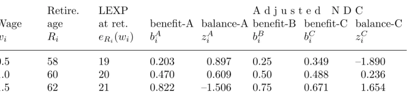
At the end of this Section, we again illustrate our results on a simple numerical example. For heterogeneous retirement ages, the simplest generalization of the LEXP–

wage function e60(w) = 20 + 6(w−1) is as follows:

eR(w) = 80−R+ 6(w−1).

Assuming that citizens spend 2/3 of their adult lives with work, R1 = 58, R2 = 60 and R3 = 62.

Table 2 reports the new results. With retirement ages depending on life expectan- cies, the ANDC contraction coefficient γ^A drops from 0.952 to 0.939 but the error of the ANDC diminishes, for example the loss z₁^A decreases from 0.952 to 0.897. With adjustment B, only the early and late retirement ages influence the benefits. Due to the proportionality of active and passive adult years, b^B_i = 0.5wi holds. With adjustment C, the loss−z₁^C = 1.22 turns to gain +1.89, while the gain−z₃^C = 0.976 changes to loss –1.654.

Table 2. NDC’s variations: heterogeneous R⁰

Retire. LEXP A d j u s t e d N D C

Wage age at ret. benefit-A balance-A benefit-B benefit-C balance-C w_i R_i e_Ri(w_i) b^A_i z^A_i b^B_i b^C_i z^C_i

0.5 58 19 0.203 0.897 0.25 0.349 –1.890

1.0 60 20 0.470 0.609 0.50 0.488 0.236

1.5 62 21 0.822 –1.506 0.75 0.671 1.654

Remark. See Table 1. Ri−L= 2[Di−L]/3, i= 1,2,3.

4. Partial wage indexation of benefits

Until now we have neglected the secular rise of real wages and the resulting conflict between relative consumption smoothing and the less than full wage indexation of ben- efits in progress. Here we model the impact of the conflict on the gains and losses. Let us assume that the real wages and the newly granted pension benefits grow uniformly with an annual factorg > 1 but the pension in progress may grow more slowly than the wages.

Consider a worker with initial wage wL who retires at the common age R, her last year real wage is related to her initial one: w_R−1 = w_Lg^R−L−1. Due to valorization (or indexation of initial benefits), her NDC wealth is equal to WR = (R−L)wR−1 = (R−L)w_Lg^R−L−1. LetD=R+e_R be the life expectancy at birth and denote byb_j the

8

real value of the benefit at age j = R, . . . , D−1. Her expected cross-sectional liability (discounted by the annual growth factor g) is equal to

WR =

D−1X

j=R

g^−j+Rbj.

Suppose that there is a scalar ι between 0 and 1, the weight of wage in benefit indexation. Then

b_j =b_j−1g^ι, where j =R+ 1, . . . , D−1.

(Note that in reality, the benefit’s growth factor is the weighted arithmetic average of wage’s and price’s growth factors, i.e. ιg+ 1−ι = (g−1)ι+ 1.) Inserting this formula to the previous one yields

(R−L)wR−1 =bR D−1X

j=R

g−(1−ι)(j−R).

To avoid superfluous separation of the analysis for ι = 1 and 0 ≤ ι < 1, we shall introduce notatione^(ι)_R for the sum:

either e⁽¹⁾_R =eR, or e^(ι)_R = 1−g^{−(1−ι)eR}

1−g^−(1−ι) for 0≤ι < 1.

Then the unadjusted NDC benefit is equal to

b^N(wR−1, R) = τ(R−L)wR−1

e^(ι)_R . (8N)

Note that the higher the weightι of wage in indexation, the greater the indexed remain- ing life expectancy e^(ι)_R and the lower the starting benefits b^N(w_R−1, R).

To take into account the heterogeneity in life expectancy, we postulate a distribution F for closing wages w_R−1 and we assume that there was no seniority wage rise, real wages rose with calendar time but at the same growth factor g for everybody. We are interested in the impact of indexation weight on the lifetime redistribution. For normalization, EwR−1 = 1.

To avoid too much repetition, we only explore adjustment A here. We shall consider the partial wage in indexation with correction A:

b^A(wR−1, R) =γ^A τ(R−L)wR−1

e^(ι)_R . (8A)

Introducing notation

e⁽¹⁾_R (w_R−1) =e_R(w_L) or e^(ι)_R (w_R−1) = 1−g^{−(1−ι)eR(wR−1)}

1−g^−(1−ι) for 0≤ι <1, (9A) 9

the lifetime balance is now

z^A(wR−1, R) =τ(R−L)wR−1−γb^N(wR−1, R)e^(ι)_R (wR−1)

=b^N(1, R)wR−1[e^(ι)_R −γ^Ae^(ι)_R (wR−1)].

Taking the expectations and equalizing the result to zero imply

0 =Ez^A(wR−1, R) =b^N(1, R)EwR−1[e^(ι)_R −γ^Ae^(ι)_R (wR−1)].

Hence

γ^A = e^(ι)_R

E[wR−1e^(ι)_R (wR−1)]. (10A) Theorem 3A. For indexed benefits, the adjusted NDC formula is given by (8A) and the correction coefficient is provided by (9A)–(10A).

We complete our Section 4 with a numerical illustration. In details, let wR−1(i) = 0.5,1,1.5 again and their common growth factor is g = 1.02. Table 3 reports the results for wage indexation: ι = 1, combined wage-price indexation: ι = 0.5 and price indexation: ι = 0. It is quite surprising that the adjustment factor is hardly sensitive to the type of indexation, it varies between 0.952 and 0.963. As the weight of wage in indexation diminishes, for every type, the initial benefit uniformly rises (and the final benefit, not shown, decreases). It is noteworthy that with wage indexation, not only the ex-ante short-lived but also the average worker contributes to the ex-ante long-lived worker’s benefit. On the other hand, with price indexation, the opposite holds.

Table 3. The impact of indexation on initial benefits and balances (A)

I n d e x a t i o n

Remaining w a g e w a g e - p r i c e p r i c e Wage LEXP benefit balance benefit balance benefit balance wi,R−1 ei b¹_i,R−1 z_i,R−1¹ b^0.5_i,R−1 z^0.5_i,R−1 b⁰_i,R−1 z⁰_i,R−1

0.5 17 0.238 0.952 0.263 0.870 0.289 0.791

1.0 20 0.476 0.476 0.525 0.420 0.577 0.369

1.5 23 0.714 –1.429 0.788 –1.290 0.866 –1.161

Remark. See Table 1, g= 1.02.

10

5. Conclusions

We have discussed three related models of NDC with three different benefit adjustments.

In Model 1, the workers only differ in wages and life expectancies but retire at the same age. Due to the positive correlation between wages and life expectancies, the scaled- down NDC strongly redistributes from the short-lived poor to the long-lived rich. In Model 2, we assume additionally that longer-lived workers also retire later, increasing the perverse redistribution. In both models, we experimented with explicit income redistribution in the pension formula. In Model 3 we return to common retirement age but introduce secular real wage rise. Diminishing the weight of the wage in indexation, the initial benefits rise and the direction of the redistribution is reversed.

In all the three models, we assumed that the workers do not react to the retirement rules and the government chooses the rules ad hoc. There is a minor exception to this approach: in the Appendix, we experiment with privately chosen savings but it has no impact of the socially optimal contribution rate. Introducing individual and social optimization in labor supply (including retirement age) and reported income, may change our results. Especially the progressivity in the pension formula may weaken the incentives to work more and retire later. Only better models can corroborate our findings.

Appendix. Optimal mix and redistribution

In this Appendix, we want to discuss the optimal mix of the NDC and flat benefits (adjustment C), i.e. their optimal shares in the basic model of Section 2. To do so, we have to define individual lifetime utility functions, which are maximized by optimally chosen individual savings. We neglect variations within the working and the retirement periods, respectively.

Let s be a nonnegative real number, representing annual saving and ρ(w) ≥ 1 be the corresponding compound interest factor. We shall approximate the true compound interest factor by the corresponding power of the annual one, (ρ[1]) as if all saving and dissaving were concentrated at the center of the accumulation and decumulation phases, respectively:

ρ(w) =ρ[1]^{(R−L+eR(w))/2}. (A.1) Then the annual young- and old-age consumption are approximated by

c= (1−τ)w−s and d =b(w) +µ(w)⁻¹ρ(w)s, where µ(w) = eR(w)

R−L. (A.2) To determine the optimal saving, one must postulate a discounted lifetime utility func- tion:

U(w, c, d) = (R−L) logc+e_R(w)δ(w) logd, (A.3) where δ(w) is the compound discount factor approximated by

δ(w) =δ[1, w]^{(R−L+eR(w))/2}, (A.4) 11

where the annual discount factor δ[1, w] is an increasing function of the wage (cf. Si- monovits, 2016).

Substituting the consumption equations (A.2) into the utility function (A.3), yields U[w, s] = (R−L)[log((1−τ)w−s) +µ(w)δ(w) log(b(w) +µ(w)⁻¹ρ(w)s)]. (A.5) Taking its derivative and equating it to zero yields the optimum condition:

U_s⁰[w, s]≈ − 1

(1−τ)w−s + δ(w)ρ(w)

b(w) +µ(w)⁻¹ρ(w)s = 0.

Then the optimal saving is as follows:

s(w) = [δ(w)(1−τ)w−b(w)ρ(w)⁻¹]+

µ(w)⁻¹+δ(w) , (A.6)

where subindex + is the positive part of the corresponding expression.

Next we define the social welfare function (cf. Feldstein, 1985 as modified in Si- monovits, 2016), replacing discounted utilities by undiscounted ones:

V[α, τ] = (R−L)E[log((1−τ)w−s(w)) +e_R(w) log(b(w) +ρ(w)s(w))]. (A.7) As is usual, we shall use relative efficiency rather than social welfare function to evaluate the optimum. Let the positive real number ε be the relative efficiency of the transfer system in terms of no transfer if by multiplying the wages in the latter the new social welfare becomes equal to that obtain in the former without changing the wages (and benefits). In formula:

V(α, τ,1) =V(0,0, ε)

Using the special properties of the logarithmic utility functions (A.5) and (A.7), V(0,0, ε) =V(0,0,1) + (R−L+e_R) logε

i.e.

ε= exp{[V(α, τ,1)−V(0,0,1)]/[R−L+eR]}.

Finally, we define the size of income redistribution through the transfer system by Dz =√

Ez².

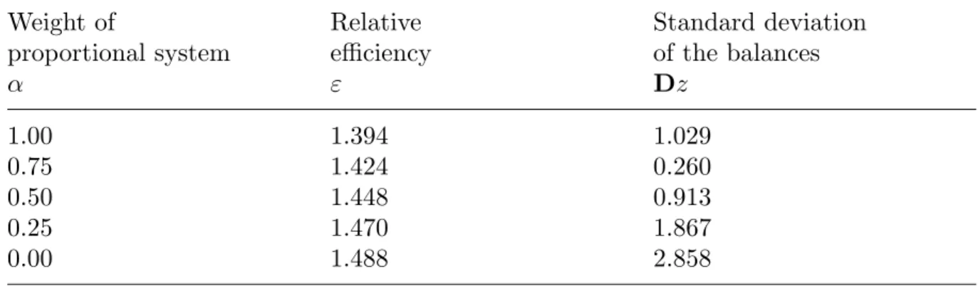
The analytical calculations would be very complicated, therefore we rest satisfied with numerical illustrations as before. Let the three annual discount factors beδ[w₁,1] = 0.9, δ[w2,1] = 0.95, δ[w3,1] = 1, and the common annual interest factor be ρ[1] = 1.02 (relative rather than real interest factor.

A simple computer calculation shows that the socially optimal contribution rate is close to τ^∗ = 0.25, regardless of the weight α. Table A1 displays the optimal efficiency and the corresponding redistribution asα sinks from 1 to 0. The relative efficiency rises from 1.394 to 1.488, while the standard deviation drops from 1.029 to 0.26 (atα = 0.75 near the minimum) and then rises again to 2.858. Depending on the importance of the two indicators, the government may choose the weight of the NDC system. We suspect

12

that if we took into account the negative impact of flat benefits on labor supply, then the social optimal share of the NDC would be higher.

Table A1. The impact of redistribution

Weight of Relative Standard deviation

proportional system efficiency of the balances

α ε Dz

1.00 1.394 1.029

0.75 1.424 0.260

0.50 1.448 0.913

0.25 1.470 1.867

0.00 1.488 2.858

Remark. τ = 0.25.

References

Auerbach, A. et al. (2017): “How the Growing Gap in Life Expectancy may Affect Retirement Benefits and Reforms,” NBER WP 23329, Cambridge, MA.

Ayuso, M., Bravo, J. M. and Holzmann, R. (2016): “Addressing Longevity Heterogene- ity in Pension Scheme Design and Reform”, IZA Discussion Paper 10378

Barr, N. and Diamond, P. (2008): Reforming Pensions: Principles and Policy Choices, Oxford, Oxford University Press.

Buchanan, J. (1968): “Social Insurance in a Growing Economy: A Proposal for Radical Reform,”National Tax Journal 21, 386–395.

Cremer, H.; Lozachmeur, J-M. and Pestieau, P. (2004): “Social Security, Variable Re- tirement and Optimal Income Taxation”, Journal of Public Economics 88, 2259–

2281.

Diamond, P. (2003): Taxation, Incomplete Markets and Social Security, Munich Lec- tures, Cambridge, MA, MIT Press.

Diamond, P. A. and Orszag, P. (2004): Saving Social Security: A Balanced Approach, Washington, D.C., Brookings Institution.

Es˝o, P. and Simonovits, A. (2002): “Designing Optimal Benefit Rules for Flexible Re- tirement”, Discussion Paper CMS-EMS 1353, Northwestern University, Evanston, IL.

Es˝o, P.; Simonovits, A. and T´oth, J. (2011): “Designing Benefit Rules for Flexible Retirement: Welfare and Redistribution”,Acta Oeconomica 61, 3–32.

Feldstein, M. S. (1985): “The Optimal Level of Social Security Benefits”, Quarterly Journal of Economics 100, 302–320.

Feldstein, M. S. (1990): “Imperfect Annuity Markets, Unintended Bequest, and the Optimal Age Structure of Social Security Benefits”, Journal of Public Economics 41,31–43.

13

Fehr, H.; Kallweit, M. and Kindermann, F. (2013): “Should Pensions be Progressive?”

European Economic Review 63, 94–116.

Fehr, H.; Kallweit, M. and Kindermann, F. (2016): “Household Formation, Female Labor Supply and Saving”,Scandinavian Journal of Economics 118, 868–911.

Holzmann, R.; Palmer, E. eds. (2006): Pension Reforms: Issues and Prospects of Non- financial Defined Contribution (NDC) Schemes. Washington, D.C., World Bank.

Holzmann, R.; Palmer, E. and Robalino, D., eds. (2012): Nonfinancial Defined Contri- bution Schemes in a Changing World. Washington, D.C., World Bank.

Legros F. (2006): “NDCs: A Comparison of French and German Point Systems,” Holz- mann and Palmer, eds. 203–238.

Liebmann, J.B. (2002): “Redistribution in the Current U.S. Social Security System”, Feldstein, M.A. and Liebmann, J.B. eds: The Distributional Aspects of Social Se- curity and Social Security Reform, Chicago, Chicago University Press, 11–48.

National Academies of Sciences, Engineering, and Medicine (2015): The Growing Gap in Life Expectancy by Income: Implications for Federal Programs and Policy Re- sponses, The National Academics Press, Washington D.C.

Pestieau, P. and Ponthiere, G. (2016): “Longevity Variation and the Welfare State”, Journal of Economic Demography 82, 207–239.

S´anchez–Romero, M. and Prskawetz, A. (2017): “Redistributive Effects of the US Pen- sion System among Individuals with Different Life Expectancy”,The Journal of the Economics of Aging 10, 51–74.

Simonovits, A. (2006): “Optimal Design of Old-Age Pension Rule with Flexible Retire- ment: The Two-Type Case”,Journal of Economics, 89, 197–222.

Simonovits, A. (2015): “Benefit–Retirement Age Schedules in Public Pension Systems”, Czech Economic and Financial Review 65, 362–376.

Simonovits, A. (2016): “Paternalism in Pension Systems”,Fecundating Thoughts: Stud- ies in Honor of Eighty-Fifth Birthday of J´anos Kornai eds. H´amori, B. and Rosta, M. 151–160, Cambridge, Cambridge Scholar Publishers.

Weinzierl, M. (2014): “Seesaws and Social Security Benefits Indexing”, Brookings Pa- pers on Economic Activity, Fall,137–196.

Whitehouse, E. and Zaidi, A. (2008): “Socioeconomic Differences in Mortality: Im- plications for Pension Policy,” OECD Social, Employment and Migration Working Papers 70, Paris OECD.

14