Cite this:Phys. Chem. Chem. Phys., 2018,20, 13224
A general formulation of the quasiclassical trajectory method for reduced-dimensionality reaction dynamics calculations†
Tibor Nagy, *aAnna Vika´r aand Gyo¨rgy Lendvay *ab
Dimension reduction by freezing the unimportant coordinates is widely used in intramolecular and reaction dynamics calculations when the solution of the accurate full-dimensional nuclear Schro¨dinger equation is not feasible. In this paper we report on a novel form of the exact classical internal- coordinate Hamiltonian for full and reduced-dimensional vibrational motion of polyatomic molecules with the purpose of using it in quasiclassical trajectory (QCT) calculations. The derivation is based on the internal to body-fixed frame transformation, as in thet-vector formalism, however it does not require the introduction of rotational variables to allow cancellation of non-physical rotations within the body- fixed frame. The formulas needed for QCT calculations: normal mode analysis and state sampling as well as for following the dynamics and normal-mode quantum number assignment at instantaneous states are presented. The procedure is demonstrated on the CH4, CD4, CH3D and CHD3isotopologs of methane using three reduced-dimensional models, which were previously used in quantum reactive scattering studies of the CH4 + X - CH3 + HX type reactions. The reduced-dimensional QCT methodology formulated this way combined with full-dimensional QCT calculations makes possible the classical validation of reduced-dimensional models that are used in the quantum mechanical description of the nuclear dynamics in reactive systems [A. Vika´ret al.,J. Phys. Chem. A, 2016,120, 5083–5093].
1. Introduction
Dimension reduction is often used in modeling phenomena in chemical physics to reduce the complexity of the model. By selecting the degrees of freedom that are relevant to the investi- gated properties of the system, one can concentrate the effort on a model whose smaller size allows one to perform a simulation at a higher level of sophistication. In molecular physics, reduced- dimensional (RD) models have been used in the description of nuclear motion both in rovibrational spectroscopy1,2as well as in molecular3–5 and reaction dynamics simulations.6–17 In both cases, the possibility of simplification is offered by the separation of time scales and the weakness of the coupling between the various modes of nuclear motion.
In vibrational spectroscopy, the semi-rigid modes are well described by the normal mode approximation18–20in which the potential and kinetic energies are considered as quadratic func- tions of Cartesian or internal coordinates and of the conjugate momenta, resp. The description of large amplitude motion (LAM), in floppy molecules, such as hindered rotor type modes, however, require a more sophisticated treatment, because the quadratic approximation does not work, often within the space swept by the zero-point motion. The frequencies of such modes are generally much smaller than those of stiffer vibrations, and the potential coupling between the fast and slow degrees of freedom is often also limited. A way to achieve a numerically feasible description of vibration of molecules with LAMs is that one reduces the dimen- sionality of the problem to those of the strongly anharmonic low- frequency modes by freezing the fast vibrations.1,2
In molecular dynamics simulation of, for example, bio- molecules in water, when a large number of solvent molecules are present, the high-frequency OH stretching vibrations require the integration time step to be small. However, their instantaneous phase has no effect on the much slower con- formational motion, thus one can freeze them,4,5which allows a significantly faster, yet realistic simulation of the system.
In reaction dynamics, the reactive event often concerns a small number of internal coordinates involving only a few atoms,
aInstitute of Materials and Environmental Chemistry, Research Centre for Natural Sciences, Hungarian Academy of Sciences, Magyar tudo´sok ko¨ru´tja 2.,
H-1117 Budapest, Hungary. E-mail: nagy.tibor@ttk.mta.hu, lendvay.gyorgy@ttk.mta.hu
bDepartment of General and Inorganic Chemistry, University of Pannonia, Egyetem u. 10, H-8800 Veszpre´m, Hungary
†Electronic supplementary information (ESI) available: Method of Lagrange multipliers for holonomic and scleronomic constraints. An efficient form of constraints allowing simple analytic gradients and Hessians. See DOI: 10.1039/
c8cp01600c
Received 12th March 2018, Accepted 17th April 2018 DOI: 10.1039/c8cp01600c
rsc.li/pccp
PAPER
Open Access Article. Published on 18 April 2018. Downloaded on 10/2/2018 7:49:34 AM. This article is licensed under a Creative Commons Attribution-NonCommercial 3.0 Unported Licence.
View Article Online
View Journal | View Issue
called active modes, and the rest are considered as ‘‘spectators’’.
Dimension reduction is possible because the potential- and often the kinematic coupling between the active and spectator modes are small. In the corresponding scattering calculation the active degrees of freedom are treated explicitly, while the coordinates of spectator modes are frozen at their values at the saddle point of the potential energy surface (PES) or at the equilibrium geometry of reactant molecules. In quantum and state-to-state quasiclassical dynamical calcula- tions it is necessary to know the quantum states of the reactants and products, for which one needs to properly characterize the vibrational motion involving only the active degrees of freedom of the reactant and product molecules, respectively. This is equivalent to the reduced-dimensional vibrational spectroscopic problem. RD models are mostly used in quantum mechanical simulations of reactions, because of the exponential growth of the computational effort with the number of degrees of freedom,1,2,6–16 but only rarely in quasiclassical trajectory (QCT) simulations, where the growth is linear.
In the QCT method,20,21the motion of the atoms is described classically and the only nuclear quantum effect considered is that the rovibrational energies of the reactant molecules are discrete. Accordingly, each rovibrational quantum state of the reactant molecules is simulated by an ensemble of semiclassi- cally quantized classical states (i.e.coordinates and momenta).
In RD reaction dynamical models the spectator degrees of free- dom are frozen during the reaction. This means that the number of vibrational degrees of freedom of the reactant and the product molecules is also reduced. Consequently, the problem of semi- classical quantization also arises when state-to-state reactivity parameters or simply state distributions of product molecules are to be determined. In what follows, the generation of classical states corresponding to a quantum state will be called the direct problem, and the determination of the quantum state corres- ponding to a given classical state will be referred to as the inverse problem.
Application of dimension reduction in QCT simulations is rather scarce. One of the reasons for this is that there is no general theory for the vibrational analysis, initial state prepara- tion and final state analysis is available. Among the few reduced- dimensional trajectory calculations performed so far, in a set only trivial reductions were applied: some of the Cartesian coordinates were simply disregarded. Lu and Hase22 applied RD models of benzene, obtained by constraining and truncating the molecule to planar C3H3and C3H moieties to prevent zero- point energy leakage from neighboring high-frequency modes during the simulation of intramolecular vibrational energy redistribution (IVR). Klossika and Schinke23 investigated the photodissociation of HNCO induced by NH vibrational excita- tion, by constraining the atoms into a plane using a reduced- dimensional analytic potential energy surface calculated only for planar arrangement of atoms.
In another set of dynamical studies the vibrations of mole- cules or fragments were completely frozen and only their relative motion was simulated. Raff and coworkers24,25applied
rigid-body dynamics to investigate rotational energy transfer between CO2 and He as well as H2. Rotational dynamics in collisions of H2O and H2 with frozen stretch vibrations were studied by Faureet al.26In some reactive scattering calculations bond lengths and angles were frozen, focusing again on rota- tional dynamics in the capture step of some bimolecular reactions (Maergoiz et al.,27 Faure et al.,28 Harding et al.29).
Harding et al.30 investigated the roaming dynamics of the photochemical decomposition of CH3CHO, where they froze the vibrations of the fragments to avoid zero-point energy leakage and the need for constructing a high-dimensional analytic PES.
More complex constraints were considered by the authors of the present paper in a recent study comparing the results of reduced- and full-dimensional (FD) quasiclassical trajectory calculations. The purpose of that work was to assess the accuracy of the Palma–Clary RD quantum dynamical model of the CH4+ H-CH3+ H2reaction,31whose FD counterpart is computationally too expensive to solve. In the present paper the general theory of reduced-dimensional QCT calculations used in that study is described. We demonstrate how the QCT method, including initial condition generation and final state can be consistently applied to RD models involving arbitrary constraints.
In the following, first we describe the three fundamental coordinate systems used in this work (Section 2.1); then in Section 2.2 we derive the vibrational Lagrangian in body-fixed Cartesian coordinates and then the vibrational Lagrangian and Hamiltonian in internal coordinates (Section 2.3). We discuss the connection of our formulation to the t-vector and s-vector formalisms in both full and reduced-dimensionality (Section 2.4).
As applications, normal mode analysis (Section 2.5) and normal mode sampling (NMS, Section 2.6) in internal coordinates and the subsequent transformation of states to laboratory frame are described. In Section 2.7, two methods of RD trajectory integra- tion are presented and compared. Section 2.8 is devoted to the inverse problem, where first the classical state given in laboratory frame is transformed to the internal coordinate system, and the normal coordinate displacements and momenta are calculated, from which the normal mode quantum numbers are determined.
The equations presented in Section 2 (apart from Section 2.4) hold not only for reduced-dimensional models but are also applicable in full dimensionality and can also serve as a basis in the derivation of RD quantum Hamiltonians. In Section 3, as a proof of principle, the method is applied to a hierarchy of three RD models of the methane molecule CZ3Y, in each of which the CZ3
group is constrained to maintain C3v symmetry. A complete reaction dynamics study based on this theory has been presented in ref. 31.
2. Theory
2.1 Frames and coordinate systems
Derivation of the classical vibrational Hamiltonian in internal coordinates starts from the full Lagrangian expressed Open Access Article. Published on 18 April 2018. Downloaded on 10/2/2018 7:49:34 AM. This article is licensed under a Creative Commons Attribution-NonCommercial 3.0 Unported Licence.
in Cartesian coordinates in a space-fixed (a.k.a. laboratory) frame:
LX;X_
¼1
2X_TMX_ VðXÞ; (1) where for anN-atomic systemX= (X1x,X1y,X1z,. . .,XNz)Tand :
X are the 3N-component coordinate and corresponding velocity column vectors, respectively, which are composed of the corres- ponding atomic coordinateRi = (Xix,Xiy,Xiz)Tand velocity :
Ri vectors. M = diag(m1,. . .,mN) is the diagonal 3N 3N mass matrix, containing the atomic masses. The classical mechanical state of the system can be given either by the coordinates and the velocities, (X,:
X) or by the coordinates and the conjugate momenta, (X,PX), the Cartesian momenta being defined as PX=M:
X.
For the description of molecular vibrations, internal coordi- nates such as valence coordinates (bond lengths, bond and torsion anglesetc.) are much more meaningful than Cartesians as the forces acting between atoms are inherently intra- molecular,i.e., they do not depend on the position and orienta- tion of the molecule. In addition, the force constants defined in terms of valence coordinates can be rationalized using chemical intuition (for example, they are roughly transferable between molecules).32 Furthermore, the use of internal coordinates is advantageous also when approximations to the Hamiltonian (e.g. quadratic- or quartic-order) are applied as they can describe large amplitude curvilinear motion more effectively than Cartesians.
In general, an internal coordinate is such a function of Cartesian coordinates, whose value is invariant under displace- ment and rotation of the molecule, thus it is necessarily formulated by using scalar (ab = aTb), and vector (a b) products of atomic Cartesian coordinate vector differences Ri Rj. Consequently, functions of internal coordinates are also internal coordinates. It is worth noting that those internal coordinates that are defined in terms of a cross product (e.g., torsion angles), change sign under mirroring the molecule through a plane (they are pseudoscalars).
For the description of the vibrating molecule one needs to definenindependent, otherwise arbitrary internal coordinates y(X) = (y1(X),. . .,yn(X))Tin terms of Cartesian coordinates. nis less than or may be equal tof= 3N6, the number of internal degrees of freedom. Ifnequalsfthen the set of internal coordi- nates is complete and the model is called full-dimensional. In reduced-dimensional models the set of irredundant internal coor- dinates is incomplete (nof) and the remainingfninternal degrees of freedom are constrained by fixing f n functions yn+1(X),. . .,yf(X) at valuesyn+1,0,. . .,yf,0. These constraint functions are generally expressed in terms of the usual valence coordinates.
For example, such a function can measure the deviation from some desired symmetry,e.g., it may be the difference of two bond lengths, which is constrained to zero. Variables yn+1(X),. . .,yf(X) expressing the constraints are formally internal coordinates, because their values should also be independent of the position and the orientation of the molecule. Note that these constrained variables are not included in vectory.
In full-dimensional models of vibrating molecules, the kinetic energy in internal coordinates is given with the help of the Wilson B matrix evaluated at the instantaneous geometry:19
B¼dy
dX; (2)
The row vectors of the (3N6)3NdimensionalBmatrix are called vibrationals-vectors1,33(si= dyi/dX). The nonredundant internal coordinatesyare defined for all values of laboratory coordinatesX, so that the inverse mass matrix
Gy,vib=BM1BT (3)
properly assigns masses to the internal coordinates and the vibrational kinetic energy in internal coordinates written as,
Ekin¼1
2pTyGy;vibpy: (4)
will be exact. However, in reduced-dimensional models (nof), theXcoordinates are interrelated by the constraints and theB matrix defined in (2) with reduced number of rows lacks the information on the corresponding constrained internal coordi- nates, which is required to disentangle them from the free ones. Consequently, such a reduced-dimensional B matrix cannot be used for the construction of the exact reduced- dimensional kinetic energy expression, unless the frozen inter- nal coordinates are orthogonal in some sense to the free ones (see ref. 1 and Section 2.4).
In order to circumvent this problem, we use the inverse transformation, which convertsfinternal coordinatesyto 3N lab Cartesian coordinates X. The inverse function X(y) and its partial derivatives by definition take into account the con- straints because they are evaluated under the condition yj(X) =yj,0forj=n+ 1,. . .,f. However, the internal coordinates do not determine the position and orientation of the molecule in the Cartesian system. To locate and orient the molecule one can utilize an intermediate body-fixed frame and an attached Cartesian coordinate system. In this auxiliary body-fixed frame the Cartesian coordinate 3N-vector and the coordinate 3-vector of atom i will be denoted by x = (x1x, x1y, x1z,. . .,xNz)T and ri= (xix,xiy,xiz,)T, respectively. The body-fixed coordinatesXare connected to the space-fixed frame by an instantaneous trans- lation and rotation, summarized in the function x(X). The definition of the intermediate frame allows us to derive the Lagrangian in internal coordinates via converting the kinetic and potential energy expressions (1) from space-fixed to body- fixed frame and (2) from body-fixed to internal frame using the inverse transformationsX(x) andx(y), respectively.
In what follows we proceed on this route in two steps. First we describe the body-fixed frame and its connection to the internal coordinates,x(y) and then its relationship to the space- fixed Cartesian frame,X(x) and show how a classical state given in internal coordinates can be transformed into the space- fixed frame.
There are many possible ways of defining a body-fixed Cartesian frame, and it depends on the system which one is Open Access Article. Published on 18 April 2018. Downloaded on 10/2/2018 7:49:34 AM. This article is licensed under a Creative Commons Attribution-NonCommercial 3.0 Unported Licence.
the most favorable. One of the simplest possibilities is that one places the origin either at the center of mass of the molecule or at one of the atoms and selects four non-coplanar atoms within the molecule and orthonormalizes three vectors pointing from one of them to the other three to obtain the basis vectors e(a=x,y,z).
The definition of the body-fixed Cartesian coordinates as a function of internal ones is given by a vector–vector function
x=x(y), (5)
whose time derivative connects the internal coordinate and the Cartesian velocities:
x:=C(y):
y. (6)
The columns of the 3N nmatrixC(y) = dx/dyare known as vibrationalt-vectors1,33,34(ti=qx/qyi).
When one knows thexcoordinates, the Cartesian coordinates of the atoms in the space-fixed frame can be obtained by considering that the body-fixed and space-fixed Cartesian frames can be brought into overlap by a translation and a rotation,i.e., thericoordinate vectors need to be rotated by matrixOframeand shifted by vectorRframeto get the space-fixed coordinatesRi:
Ri=Rframe+Oframeri. (7) The atomic velocity :
Riis obtained from that in the body-fixed frame (:
x) by differentiating eqn (7) with respect to time:
R:i= :
Rframe+ :
Oframeri+Oframe:
ri, (8) where :
Rframeis the velocity of the body-fixed frame with respect to the space-fixed one. To get :
Oframe, one needs to take into account that the body-fixed frame may rotate around its origin with angular velocityxframe. The total time derivative of the rotation matrixOframe is then :
Oframe=xframeOframe, where the cross product ofoframe and matrixOframeneeds to be evaluated column by column. With this, the atomic velocityRiin the space-fixed Cartesian frame is:
R:i= :
Rframe+ (xframeOframe)ri+Oframe
r:i. (9) Unless special care is taken, the body-fixed frame does not move together with the molecule: its instantaneous linear (:
Rframe) and angular velocities (xframe) differ from those of the molecule in the space-fixed frame. For example, when the body- fixed frame for a vibrating water molecule (H2O) is selected to be centered at theOatom with thex-axis parallel to H1H2, then the linear velocity of the origin of the frame is not identical to that of the center of mass, and the antisymmetric OH stretch vibration generates angular motion of the molecule (see Fig. 1).
Obviously, the physically correct description of motion requires both the displacements of the atoms of the molecule in the body-fixed frame and translation + rotation of the body- fixed frame in the lab frame. Consequently, the transformation of internal coordinates and momenta to body-fixed frames according to eqn (5) and (6) usually generates unphysical (often referred to as spurious35) translation and rotation.
When the focus is on the vibrational motion of a molecule, however, the general procedure is that the motion of the
body-fixed frame is disregarded and extra steps are made to eliminate the spurious rotation and translation which would falsify the effective masses assigned to internal coordinates. In thet-vector formalism the cancellation of spurious rotation is achieved by the introduction of rotational coordinates when vibrational energy levels are calculated.1,2
In classical mechanics, when a vibrational state is generated by normal mode sampling, the molecule can artificially be cleared of these unwanted velocities.36In general, it is desirable to avoid the appearance of the unphysical translational and rotational terms, a novel way of which is proposed in the following sections.
2.2 Vibrational Lagrangian in body-fixed Cartesian coordinates
To derive the pure vibrational Lagrangian Lx,vib(x,:
x) in body- fixed Cartesian coordinates, first the LagrangianLx(x,:
x) for the non-translating and non-rotating body-fixed frame is obtained.
To achieve this, one substitutes eqn (7) and (9) into eqn (1) and eliminates the rotational and translational motion of the body- fixed frame by setting :
Rframe= 0 andxframe= 0. Exploiting that matrixMis diagonal and matrix Oframeis unitary, the kinetic energy function in the new coordinates can be transformed into the same form in body-fixed Cartesian coordinates as it was in the lab Cartesian frame, in accordance with the expectations.
The form of the potential energy function will also remain the same because it is a function of internal coordinates only, which are defined with dot and cross products (brief common notation:), that are also left unchanged by_ Oframe.
Lxðx;x_Þ ¼LXðxÞ;X x;_ð x_Þ; _Rframe¼0;xframe¼0
¼ XN
i¼1
1
2miR_TiR_iV RjRk
_ðRlRmÞ
¼ XN
i¼1
1
2mir_Ti_riV rjrk
_ðrlrmÞ
¼1
2x_TMx_VðxÞ:
(10) Fig. 1 Schematic drawing of the motion of a water molecule (H1OH2) in a specific body-fixed frame, which is centered at the O atom with thex-axis parallel to the H1H2line. (a) The equilibrium geometry with space-fixed displacements (blue arrows) due to antisymmetric stretch vibration. (b) The distorted molecule and the body-fixed frame aligned according to the new H–H axis. (c) The distorted molecule when the body-fixed frame is aligned as in (a), showing the corresponding atomic displacements in the body- fixed frame, which result in a clockwise rotated structure whose center of mass (CM) is displaced upward and to the left in the body-fixed frame.
Open Access Article. Published on 18 April 2018. Downloaded on 10/2/2018 7:49:34 AM. This article is licensed under a Creative Commons Attribution-NonCommercial 3.0 Unported Licence.
The curly bracket refers to the sets of products involving the atomic indices (j, k, l, m) that are used in the definition of internal coordinates.
We would like to obtain the pure vibrational Lagrangian.
For this we need to decompose the kinetic energy into sepa- rate vibrational as well as translational and rotational parts.
If one introduces mass-scaled coordinates ˜x = M1/2x, the quadratic form of the kinetic energy expressed in the body- fixed Cartesian frame (Tx) reduces to the square of the mass- scaled velocity vector x~_ . This form is advantageous, because it allows one to decompose the instantaneous mass-scaled velocity vector into orthogonal translational, rotational and vibrational parts (we show later how). Once these compo- nents, x~_trans, ~x_rot and ~x_vib are available, the kinetic energy can also be broken down into the correspondingTtrans,Trot
andTvibterms:
Tx ¼1 2 M12x_
T
M12x_¼1 2~x_2¼1
2x~_trans2þx~_rot2þx~_vib2
¼TtransþTrotþTvib:
(11)
Consequently, the vibrational part can be obtained by elim- inating the components of the mass-scaled velocity that corre- spond to translation and rotation,i.e., projecting the velocities onto the complementary and orthogonal, instantaneous (geometry-dependent) vibrational subspace. If the 3N 3N matrix that performs the desired projection in the space of mass-scaled velocities is denoted byPvib(x), the pure vibrational Lagrangian can be formally written as:
Lx;vibðx;x_Þ ¼1
2 PvibðxÞM12x_
T
PvibðxÞM12x_VðxÞ: (12)
Utilizing the fact that the orthogonal projectors onto the translational and rotational subspaces, Ptrans and Prot(x), can be easily found (see below) and their sum is complementary to Pvib(x), we definePvib(x) in terms of them:
Pvib(x) =EPtransProt(x), (13) where E is the 3N 3N unit matrix. In the following we define the basis vectors of the translational and rotational subspaces and using them, we construct the corresponding projectors.
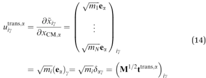
The translational subspace of mass-scaled displacements and velocities is spanned by the three 3N-component translational basis vectorsutrans,a(a=x,y,z):
utrans;aig ¼ @x~ig
@xCM;a¼ ffiffiffiffiffiffi m1 p ea
... ffiffiffiffiffiffiffi mN p ea 0 BB BB
@
1 CC CC A
ig
¼pffiffiffiffiffimi ea ð Þg¼pffiffiffiffiffimi
dag¼M1=2ttrans;a
ig
(14)
utrans,aig denotes theg(g=x,y,z) component of the mass-scaled displacement of atomiduring translation of the whole mole- cule along axisa(see Fig. 2a–c).dag is the Kronecker symbol, which is evaluated usingx= 1,y= 2,z= 3 assignments to the possible values of its indices aandg. The translational basis vectors are related to translational t-vectors (ttrans,a) by mass- scaling. The translational basis vectors only depend on the masses and are independent of the geometry and also of the choice of the origin of the body-fixed frame. Consequently, the translational subspace is the same at all geometries and thus it includes all finite mass-scaled translations of the molecule.
The rotational subspace is spanned by the three 3N-component rotational basis vectorsurot,a(x), which describe the relative magni- tude of the mass-scaled displacements of atoms due to an infinitesimal rotation of the molecule around theaprincipal axis (PA) of the instantaneous moment of inertia tensor (a= 1, 2, 3, but notx,y,z). Rotational basis vectors can be calculated from the orthonormal unit vectors of principal axes ePAa (given in the body-fixed frame) and the instantaneous position vectors of atomsqi:=rirCM(i= 1,. . .,N) relative to the center of mass of the molecule,rCM:
urot;aig ðxÞ ¼ @x~ig
@jPAa
¼ ffiffiffiffiffiffi m1
p ePAa q1
... ffiffiffiffiffiffiffi mN
p ePAa qN 0
BB BB
@
1 CC CC A
ig
¼pffiffiffiffiffimi
ePAa qi
g
¼pffiffiffiffiffimi X
s¼x;y;z
X
t¼x;y;z
egstePAasrit¼ M1=2trot;a
ig: (15)
urot,aig characterizes the relative magnitude of thegcomponent (g=x,y,z) of the mass-scaled displacement of atomiwhen the
Fig. 2 The three translational (a–c), two rotational (d and e) and one vibrational (f) normalized basis vectors of a homonuclear diatomic molecule (H2, O2,etc.) at a given orientation. The Cartesian coordinate system and the indices of atoms are shown in the leftmost panel. In panels (d and e), the center of mass (CM) is shown in blue, and the unit vectors along the principal axes are shown in red.
Open Access Article. Published on 18 April 2018. Downloaded on 10/2/2018 7:49:34 AM. This article is licensed under a Creative Commons Attribution-NonCommercial 3.0 Unported Licence.
molecule is rotated infinitesimally around the a (= 1, 2, 3) principal axis (see Fig. 2d and e). The angle of the rotation aroundePAa is denoted byjPAa .egstis the Levi-Civita tensor which is evaluated using assignmentsx= 1,y= 2,z= 3 regarding the possible values of its indicesg,s andt. The rotational basis vectors are related to rotationalt-vectors (trot,a) corresponding to rotations around the principal axes by mass-scaling. The rotational basis vectors depend on the geometry. Thus they can be used to describe only infinitesimal mass-scaled displace- ments of atoms during the rotation of the molecule. The translational and the rotational basis vectors are orthogonal to each other, and by normalizing them an orthonormal set of translational and rotational basis vectors,utrans,a0 andurot,a0 (x) can be obtained. The proof of orthogonality and the derivation of the squared norms of the basis vectors are presented in the Appendix.
The instantaneous vibrational subspace, which is orthogonal to the translational and rotational subspaces, also depends on the geometry, thus it will span only infinitesimal mass-scaled displacements during the vibration of the molecule. When the shape and the orientation of the molecule do not change during its motion, for example, during the symmetric stretch vibration of CH4or during the translation of any molecule, the rotational and vibrational subspaces will not change either. A possible orthonormal basis (uvib,i0 (xe),i= 1,. . .,f) of the vibrational sub- space at equilibrium geometry (xe) is formed by the vibrational normal mode eigenvectors (see Fig. 2f), which are obtained from harmonic vibrational analysis done in Cartesian frame atxeand are mass-scaled by definition. The orthonormal basis vectors of the translational, rotational and vibrational subspaces of a homonuclear diatomic molecule are summarized in Fig. 2.
The orthogonal projection matrices Ptrans and Prot(x) can be defined as dyadic productsab¼abT
of the relevant basis vectors:
Ptrans¼ X
a¼x;y;z
utrans;a0 utrans;a;T0 ; (16)
ProtðxÞ ¼X3
a¼1
urot;a0 ðxÞurot;a;T0 ðxÞ: (17) These are the projectors to be used in eqn (13) to generate the orthogonal projection matrixPvib(x) onto the complementary, vibrational subspace. MatrixPvib(x), being an orthogonal pro- jector, is idempotent (Pvib2(x) =Pvib(x)) and symmetric while the mass matrixM is diagonal. Consequently, by introducing an effective vibrational mass matrix:
Mvib(x) =M1/2Pvib(x)M1/2, (18) which is geometry dependent and dense as opposed to matrix M, the Lagrangian in eqn (12) can be rewritten in the form:
Lx;vibðx;xÞ ¼_ 1
2x_TMvibðxÞx_VðxÞ: (19) Matrix Mvib(x) is singular, since it assigns non-zero masses only to the motion within the vibrational subspace, which has
fewer dimensions than 3N. Momenta px,vib canonically conjugate to coordinatesxare obtained by differentiating the Lagrangian:
px;vib¼@Lx;vibðx;xÞ_
@x_ ¼MvibðxÞx:_ (20)
While the velocity vector :
x may describe translation and rotation in addition to vibration of the molecule in the body-fixed frame, the momentum vector px,vib describes only vibrations, because it is obtained by the singular mass matrixMvib(x). Thus, the Euler–Lagrange equations of motion cannot describe translation and rotation within the body-fixed frame.
We note that the present derivations are similar to the projection method proposed by Milleret al.37and Szalay used projections for the approximate decomposition of the kinetic energy in the Eckart frame.38The difference is that we apply the exact decomposition of the instantaneous kinetic energy.
2.3 Vibrational Hamiltonian in internal coordinates
The vibrational Lagrangian in internal coordinatesyand velo- cities :
y can be obtained from eqn (19) using the transforma- tions in eqn (5) and (6):
Ly;vibðy;yÞ ¼_ 1
2ðCðyÞyÞ_ TMvibðxðyÞÞCðyÞy_VðxðyÞÞ
¼1
2y_TMy;vibðyÞ_yVyðyÞ:
(21)
Here we introduced the potential energyVy(y) =V(x(y)) as well as the n n vibrational mass matrix, My,vib as a function of internal coordinatesy:
My,vib(y) =CT(y)M1/2Pvib(x(y))M1/2C(y). (22) At this point, it becomes obvious that by projecting onto the vibrational subspace, we cancel the spurious translation and rotation in the body-fixed frame and the masses corresponding to them will not contaminate the mass matrix assigned to the internal coordinates, which would unphysically increase the matrix elements. Without the projection, for example, harmonic vibrational analysis would give incorrect, reduced frequencies for some of the normal modes.
Eqn (22) applies as it is regardless whethern=forno f.
Its form implies that in reduced-dimensional models the reduced- dimensionalMy,vib(y) matrix can also be obtained from the full- dimensional My,vibby simply deleting the rows and columns corresponding to the constrained internal coordinates.
Momenta canonically conjugate to the internal coordinates are obtained as:
py¼@Ly;vibðy;yÞ_
@y_ ¼My;vibðyÞy;_ (23)
and the velocity:
yas a function ofyandpywill be
y:=My,vib1(y)py=Gy,vib(y)py. (24) Here, thenndimensionalGy,vib(y) matrix is the inverse of the non-singularMy,vib(y) matrix. Applying Legendre transformation Open Access Article. Published on 18 April 2018. Downloaded on 10/2/2018 7:49:34 AM. This article is licensed under a Creative Commons Attribution-NonCommercial 3.0 Unported Licence.
to the Lagrangian, one can obtain the vibrational Hamiltonian in internal coordinates:
Hy;viby;py
¼pTyy y;_ py
Ly;viby;y y;p_ y
¼1
2pTyGy;vibðyÞpyþVyðyÞ:
(25)
This form is correct in any nonredundant set of internal coordinates, be it reduced (nof) or complete (n=f).
2.4 Connection with the t-vector and the s-vector formalisms In the previous two sections we derived the vibrational kinetic energy in internal coordinates by introducing the body-fixed framexand using the inverses of the arbitrarily definedx(X) andy(x) transformations. In this section we show the relation- ship of our method to those that are generally used for this purpose in the literature, one those based on theX-ytrans- formation1,33,39 (s-vector formalism) as well as on they - x transformation1,40(t-vector formalism).
The s-vector formalism provides the exact vibrational Hamiltonian for the full-dimensional vibrational problem. To derive the reduced-dimensional kinetic energy and the mass matrices using theX-ytransformation, it is necessary to extend the set of variables to a full set of internal variables and first construct the full-dimensionalGy,vib(see eqn (3)). Then one can either calculate the full-dimensionalMy,vibby inversion, then delete rows and columns and invert again, or directly correct the block of Gy,vibcorresponding to the kept variables (ref. 19, Appendix IX) to account for the effect of the constrained ones.
The t-vector formalism requires the definition of a body- fixed frame (e.g., Eckart frame41), which is rarely the absolute co-rotating frame. To compensate for the arising spurious rotation during the change of internal coordinates of the molecule, rotational coordinates need to be introduced and a rovibrational Hamiltonian has to be constructed to make possible the exact description of the vibrational problem. The reduced-dimensional Hamiltonian is directly obtained by using only those vibrationalt-vectors which belong to non-constrained internal variables.
The method presented in this work is analogous to the t-vector formalism also in the sense that both are based on the dx/dyderivatives and allow the direct construction of a reduced- dimensional Hamiltonian. However, instead of introducing rota- tional variables, our method exploits the orthogonality of the mass-scaled translational and (instantaneous) rotational basis vectors (3N-component) to vibrational ones so that rotation and translation are exactly removed. This approach provides a pure vibrational kinetic energy expression equivalent with the one provided with thes-vector formalism.
It can be shown that the inverse mass matrixGy,vibin the s-vector formalism (eqn (3)) is the inverse of theMy,vibmass matrix in eqn (22) and that this does not hold for the reduced- dimensional case as the pure-vibrational infinitesimal mass- scaled Cartesian displacement vectors corresponding to the various internal coordinates are not orthogonal to each other in general. This also implies that thes-vector formalism in full
internal dimensionality is in fact a reduced-dimensional approximation, because it considers only vibrations and trans- lational and rotational coordinates are simply omitted. This raises the question how it can be exact for vibrations. The reason for this is the inherent orthogonality of vibrations to rotations and translations in mass-scaled infinitesimal displace- ment space.
2.5 Normal mode analysis in internal coordinates
During normal mode analysis the vibration of the molecule is approximately decomposed into independent harmonic oscil- lators using the harmonic approximation to the kinetic and potential energy expressions. The harmonic approximation to the Lagrangian in internal coordinates in the neighborhood of a stationary pointy0can be obtained by replacing theMy,vib(y) matrix function with its value aty0,My,vib,0=My,vib(y0), approxi- mating the potential energy to second order around y0, and setting its zero level to that at geometryy0:
Lharmy;vibðy;yÞ ¼_ 1
2y_TMy;vib;0y_1
2ðyy0ÞTFy;0ðyy0Þ: (26) HereFy,0=Vy00(y0) is the force constant matrix. This generally proves to be a good approximation to the Lagrangian at low energies in semi-rigid molecules, where no internal rotations or other large amplitude motion can take place.
From here on one can follow the standard procedure of normal mode analysis. After introducing mass-scaled vectors of deformationy˜=My,vib,01/2(y y0) and velocity~y_¼My;vib;01=2y_ and theF˜y,0=Gy,vib,01/2Fy,0Gy,vib,01/2mass-scaled force constant matrix (where Gy,vib,0 = My,vib,01) one solves its F˜y,0U = UK eigenproblem. MatrixF˜y,0is symmetric, thus allneigenvalues li(in matrixK= diag(l1,. . .,ln)) are real and the eigenvectors (i.e.columns ofU) can be chosen to be orthonormal. Ify0is a potential minimum, all eigenvalues are positive, whereas for a kth-order saddle point k of them are negative. The vector of normal-mode deformation coordinatesQ= (Q1,. . .,Qn)Tand the canonically conjugate momentum vectorP= (P1,. . .,Pn)T(in fact, the normal-mode velocity vector :
Q) are defined as:
Q=UT˜y=UTMy,vib,01/2(yy0), (27) P= :
Q=UT˜y=UTMy,vib,01/2:
y. (28)
In normal coordinates both the Lagrangian and the Hamiltonian (i.e.energy) decompose into sums ofnharmonic oscillator (HO) terms:
Hharm;i1D ðQi;PiÞ ¼Eharm;i1D ¼1 2Pi2þ1
2oi2Qi2
¼1 2Q_i2þ1
2oi2Qi2:
(29)
The normal mode frequencies can be obtained asoi=li1/2. 2.6 Normal mode sampling
The purpose of normal mode sampling is the generation of a set of classical states corresponding to a preselected vibrational state of a reactant molecule that will serve as initial conditions Open Access Article. Published on 18 April 2018. Downloaded on 10/2/2018 7:49:34 AM. This article is licensed under a Creative Commons Attribution-NonCommercial 3.0 Unported Licence.
for collision or intramolecular trajectories. In QCT calculations, the initial states of molecules are usually generated by assuming that vibration and rotation are separable and the vibrations are well described by the normal mode approximation. The procedure for normal mode sampling is well known for full-dimensional models, but without the proper RD normal mode analysis, it cannot be used in reduced dimensionality. In normal mode sampling it is assumed that the vibrating molecule can be well approximated as a set of independent normal oscillators with ndistinct quantum numbersv1,. . .,vn(nconstants of motion).
In quasiclassical quantization, normal coordinate and momentum amplitudes (Qi,max,Pi,max= :
Qi,max) of each normal mode oscillator are set so that the energy of the oscillator (E1Dharm,i) matches that of the corresponding quantum harmonic oscillator in a givenvi
quantum state:
E1Dharm;i ¼1
2oi2Qi;max2¼1
2Pi;max2¼1 2Q_i;max2
¼hoi viþ1 2
:
(30)
For the generation of classical states (Q,P), a random initial phaseji,0is selected from a uniform distribution in the [0,2p) interval for each vibrational mode, and then the normal mode coordinate and velocity of normal oscillatorican be calculated according to:
Qi=Qi,maxcosji,0, (31)
Pi= : Qi=:
Qi,maxsinji,0. (32)
The corresponding classical state (y,:
y) in internal coordinates can be obtained by inverting eqn (27) and (28):
y=y0+Gy,vib,01/2UQ, (33)
y:=Gy,vib,01/2UP=Gy,vib,01/2U:
Q. (34)
The resulting classical state (y,:
y) is the appropriate initial state if one intends to follow the time evolution of the system using the Euler–Lagrange or Newton equations of motion. If one would like to describe the same dynamics in the more con- venient Hamiltonian formalism (see Section 2.7.1), then the initial state should be expressed in internal coordinates and the conjugate momenta (y,py), where the momenta are obtained from eqn (23) with the mass matrixMy,vib(y) calculated at the instantaneous geometryy.
When the trajectory integration is to be performed in Cartesian coordinates, the state (y,:
y) needs to be transformed to the body-fixed Cartesian frame and one should ensure that the unphysical translation and rotation generated during trans- formations in eqn (5) and (6) are removed. To obtain the pure vibrational classical state (x,px,vib), the body-fixed Cartesian coordinatesx are calculated fromyusing eqn (5); the corres- ponding Cartesian momenta describing vibration only are found by transforming:
yto:
xwith matrixC(y) and finally topx,vibwith matrixMvib(x) using eqn (6) and (20), respectively:
px,vib=Mvib(x):
x=Mvib(x(y))C(y):
y. (35)
The point here is that the geometry-dependent mass matrix Mvib(x), which assigns mass only to vibrations, guarantees that the resulting classical states (x,px,vib) will have zero center-of- mass momentum and angular momentum. The coordinate and velocity conversion equations also ensure that Cartesian coor- dinatesx, velocities :
xand momentapx,vibfulfill the equations of geometrical constraints (yn+1(x) = yn+1,0,. . .,yf(x) = yf,0) and their time derivatives (see Section 2.7.2).
The ensemble of classical states (x,px,vib) in Cartesian coordi- nates, which corresponds to the pre-selected vibrational quan- tum state of the reduced-dimensional model of the reactant molecule is generated by carrying out the sampling procedure many times with different random phases in eqn (31) and (32).
It should be noted that the ensemble obtained this way is not monoenergetic. In QCT calculations the nonrotating molecules are randomly oriented before collision. If a rovibrational state is to be generated, then the molecule’s angular momentum is also set to that of the desired quantum state. The obtained classical states are in laboratory Cartesian frame and thereby they can be used in the definition of initial conditions of the molecule (X,PX), for QCT calculations.
The standard method to prepare monoenergetic ro-vibrating ensembles by iterative rescaling of deformations and momenta and angular momentum vector adjustment after normal mode sampling has been proposed by Hase and coworkers.42 That method can be generalized to reduced-dimensional models.
What remains the same is that the scaling factor is determined in the lab frame. The important difference is that in the full- dimensional model the scaling factor can be applied to scale the lab-frame deformations and momenta. In RD models the rescaling step needs to be performed in internal coordinates, because otherwise it would violate the constraints. It should be noted that the ensembles generated this way are not stationary when allowed to evolve on the real, anharmonic PES.21Mono- energetic, stationary and accurately quantized ensembles of classical states representing a rovibrational quantum state can be generated by applying the adiabatic principle of classical mechanics. A generalized version of the adiabatic switching method, which accurately includes anharmonicity and coupling of vibrations, has recently been shown to perform well for polyatomic molecules.43 The method has also been extended to generate ensembles corresponding to rovibrational quantum states.
2.7 Dynamics in reduced dimensionality
In reduced-dimensional classical trajectory calculations the equations of motion for the intramolecular motion of molecules have to guarantee the fulfillment of the constraints prescribed by the model. In the following, we discuss two choices: the applica- tion of equations of motion in internal coordinates and the integration of the equations of motion in lab Cartesian frame, supplemented by constraint forces. Integration in internal coor- dinates is more appropriate for the description of a vibrating molecule, whereas the equations presented for integration in 3N Cartesians are equally applicable both to pure bound motion and to scattering problems.
Open Access Article. Published on 18 April 2018. Downloaded on 10/2/2018 7:49:34 AM. This article is licensed under a Creative Commons Attribution-NonCommercial 3.0 Unported Licence.
2.7.1 Equations of motion in internal coordinates.
Hamiltonian equations of the pure vibrational motion in internal coordinates can be derived from the Hamiltonian in eqn (25).
p_y¼
@Hy;viby;py
@y ¼ 1
2pTyGy;vib
0ðyÞpyVy0ðyÞ; (36)
_ y¼
@Hy;viby;py
@py ¼Gy;vibðyÞpy: (37)
Rank-3 tensor Gy,vib0(y) and vector Vy0(y) are the coordinate derivatives of the inverse mass matrixGy,vib(y) and the potential energy Vy(y). The initial conditions of the motion can be obtained via eqn (33) and (34) and formula py = My,vib(y)y.: When vibrational dynamics are simulated, internal to body- fixed frame transformation and projection onto the vibrational subspace have to be performed several times at every integra- tion step for the evaluation ofGy,vib(y),Gy,vib0(y) andVy0(y) (see eqn (5), (6), (22) and (24)). The generally involved calculation of the rank-3Gy,vib0(y) derivative tensor can be sped up by using some analytical transformations (see ESI†). A more serious drawback of using internal coordinates is that they may become indeterminate and in that neighborhood they change very steeply. At these points the coordinate transformation in eqn (5) or its inverse has singularities, which can cause signi- ficant numerical errors during the solution of the equations of motion. For example, such a singularity arises for 3D polar coordinates (r,y,j) at small (y= 01) and large (y= 1801) polar angles wherejmay change very quickly during dynamics. With careful selection of the body-fixed frame and the set of internal coordinates one can achieve that the singularities of the transfor- mation equations (eqn (5) and (6)) will be at highly deformed geometries which are not sampled by normal mode state prepara- tion and not visited during the vibration of the molecule. It is important to emphasize that eqn (36) and (37) describe the vibration of non-rotating molecules only.
2.7.2 Equations of motion with constraints in space-fixed Cartesian coordinates. During the internal motion of floppy molecules, as well as in loose clusters and chemical reactions, where bonds get broken and formed, highly-deformed geome- tries are visited and the moieties of reactant molecules can have arbitrary orientation with respect to each other. For such systems, it is preferable to simulate the reduced-dimensional dynamics by integrating the equations of motion in the full set of 3N lab Cartesian coordinates (X) and enforcing the restrictions in the internal degrees of freedom by constraint forces. To derive constraint forces, we introduce functionsgi(X) (i= 1,. . .,f n) as the deviations of functionsyn+i(X) from their corresponding frozen valuesyn+i,0. The equations of constraints are obtained by equating thegi(X) functions to zero.
gi(X) :=yn+i(X)yn+i,0= 0 i= 1,. . .,fn. (38) These constraints are holonomic as they depend only on the position coordinates (but not on their time derivatives) and are scleronomic as they do not depend on time explicitly. They are
expected to be fulfilled all along a trajectory, implying that their time derivatives must also be zero:
g:i(X,: X) =rTgi
X: =rTgiM1PX= 0 i= 1,. . .,fn, (39) which serve as constraint equations for the velocities :
X and momentaPX. Consequently, a mechanical state, which is fully characterized either by (X,:
X) or (X,PX), should fulfill eqn (38) and (39) simultaneously. The 3N-component constraint force arising from constraintiin eqn (39) is necessarily parallel to gradientrgi, because it confines the allowed motion (velocity:
X) to a (3N1)-dimensional surface orthogonal torgi. Consequently, each constraint forceFconstri is expressed as being proportional to rgiwhich, multiplied by Lagrange multipliersli(i= 1,. . .,fn) are added to Hamilton’s equations for momenta, supplementing there the potential forces:
P_X¼ rVþXfn
i¼1
Fconstri ¼ rVþXfn
i¼1
lirgi: (40) The Hamiltonian equations of motion for the coordinates remain the same (:
X = M1PX) since the constraints in eqn (38) are holonomic. The Lagrange multipliers need to be calculated at every time step of trajectory integrationviaa set of linear equations. An excellent description of how the Lagrange multipliers are determined in practice can be found in ref. 3, 4 and 20. For completeness, the equations with the present notations are summarized in the ESI.†
2.7.3 Comparison of the computational aspects of the two descriptions. Usually the most expensive part of trajectory simulations is the evaluation of potential gradients. If no analytical gradients of the potential energy are available, then they need to be evaluated numerically with finite difference formulae, whose computational cost scales linearly with the number of gradient components. When nonredundant internal coordinates are used, some computational savings come from the reduced number (fo3N6) of gradient components in theVy0(y) potential gradient compared to the full-dimensional Cartesian problem (3N). On the other hand, simulation of the dynamics in irredundant internal coordinates requires repeated evaluation of rank-3 tensor Gy,vib0(y), which can be expensive unless analytical first and second derivatives (matricesC(y) andC0(y)) of the coordinate transformationx(y) are available. Analytical derivation of matrixCcan be compli- cated and requires non-negligible human effort even when computer algebra packages are employed, and even when the derivatives are available, their evaluation may require numerous algebraic operations.
In the alternative method, integration of the equations of motion in Cartesian coordinates under the control of con- straints, at least 6 more potential gradient components need to be evaluated; in addition, the constraint forces need to be determined. Yet, the application of Cartesian coordinates together with constraints can be overall cheaper than using internal coordinates, especially when analytic first derivatives of the PES, and first and second analytic derivatives of the constraints are available.
Open Access Article. Published on 18 April 2018. Downloaded on 10/2/2018 7:49:34 AM. This article is licensed under a Creative Commons Attribution-NonCommercial 3.0 Unported Licence.
An additional aspect is the accuracy to which the constraints prescribed by the reduced-dimensional model are fulfilled.
Integrating in internal coordinates automatically satisfies these constraints. On the other hand, when full-dimensional Cartesian coordinates are used, the constraints are enforced numerically, so that their fulfillment (eqn (38) and (39)) depends on the accuracy of the numerical procedure. Accordingly, in long simulations it is desirable to check regularly how well the constraints are met. If any of them is violated significantly, fulfillment of them can be reestablished by minimizing to zero the sum of the properly scaled squares of the left hand sides of eqn (38) and (39).
2.8 Assignment of normal mode quantum numbers to reduced-dimensional classical states
Solution of the inverse problem, determination of normal mode quantum numbers corresponding to a reduced-dimensional classical state of the molecule is needed when product-state resolved properties are calculated for bimolecular reactions or when the classical evolution of vibrationally excited states of molecules is of interest. Depending on which of the two sets of Hamiltonian equations of motion (Section 2.7) were used for trajectory integration, the classical state of the system is provided either in nonredundant internal coordinates and momenta (y,py) or in space-fixed Cartesian coordinates and momenta (X,PX) fulfilling constraints in eqn (38) and (39).
In the former case, since the normal mode analysis of the reduced-dimensional model is done in internal coordinates (see Section 2.5), the state expressed as (y,:
y = Gy,vib(y)py) can be directly used for quantum number assignment as described below. However, when the state is given in Cartesians,XandPX need to be converted to internal coordinates and velocities.
Coordinatesycan be computed directly from theXcoordinates, which fulfill thefnconstraints given in eqn (38), using the definition of the internal coordinatesy(X). Velocities of internal coordinates can be obtained by either numerical derivation along the trajectory or analytical differentiation utilizing the reduced-dimensional variant of Wilson’sBmatrix (see eqn (2)) and the Cartesian velocities :
X=M1PX: yðtÞ ¼_ lim
Dt!0
y XðtÞ þ XðtÞDt_
y XðtÞð Þ Dt
¼ dy dXjXðtÞ
XðtÞ ¼_ BðXðtÞÞM1PXðtÞ
(41)
It is important to point out that, while the reduced- dimensional Bmatrix cannot be used for the construction of Gy,vibdue to the non-orthogonality of internal coordinates (see Section 2.4), it can be applied to transform Cartesian velocities to internal coordinate velocities if and only if they fulfill the constraints.
Once the state is given as (y,:
y), the normal mode coordinates and momenta can be calculated by inverting eqn (33) and (34):
Q=UTMy,vib,01/2(yy0), (42)
P= :
Q=UTMy,vib,01/2:
y. (43)
The E1Dharm,i mode energies can be calculated from the instantaneous normal coordinates and momentaviaeqn (29).
The quantum numbersviare obtained from the energy corres- ponding to each vibrational mode using the inverse of the harmonic oscillator quantization rule (eqn (30)).
ni¼E1Dharm;i hoi 1
2 (44)
Note that the vibrational quantum numbers ni obtained this way are in general not integer numbers and because of this, the assignment of a quantum state to the given classical one is not unequivocal, and various tricks are generally used to do it (see, e.g.ref. 44 and 45).
3. Results
3.1 Three reduced-dimensional models of methane
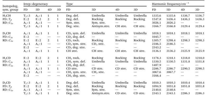
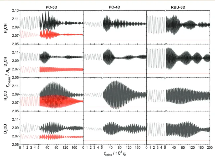
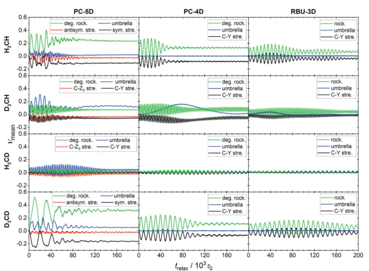
In this section we apply the methods described above to normal mode analysis and sampling in various reduced-dimensional models of methane used in ref. 31 to study RD QCT reaction dynamics calculations of the reaction, which is the most complicated type of reaction for which exact RD quantum mechanical scattering calculations are available.13,46,47 The RD model with the fewest restrictions is the one proposed by Palma and Clary (in the following, PC):9,10the only constraint is that the CZ3group keepsC3vsymmetry. The model and a series of its versions with additional constraints have been used in numerous quantum scattering simulations. In order to assess the performance of the RD models, Vika´ret al.31compared the results of (quasi)classical trajectory simulations obtained with the Palma–Clary and the full-dimensional models of the CH4+ H-CH3+ H2reaction with various CH4isotopologs. We just mention in passing that the PC model was found to give good results in many cases, but its performance proved to depend on the quality of the potential energy surface and the mass combination.31
Starting from the PC model, one can design a hierarchy of reduced-dimensional models for methane, in each of which the geometry of the CZ3moiety is constrained to maintainC3vpoint group symmetry and by freezing additional types of motion, its internal degrees of freedom are reduced fromf= 9 to 5, 4 or 3.
Since the three Z atoms are treated as equivalent, such models are suitable for the description of methane isotopologs CHnD4nwith n= 0, 1, 3, 4 but not for CH2D2. In Fig. 3 the models with their reduced sets of internal variables and the attached body-fixed Cartesian frame are shown.
The latter was defined for all models in the same way: the origin was placed at the carbon atom and the axes were determined by the constrained CZ3moiety:zaxis is along the C3vaxis,xaxis within the YCZ1plane, forming an acute angle with the CZ1vector, and theyaxis is chosen to ensure that the coordinate system is right-handed.
In the ‘‘full’’ Palma–Clary model9(Fig. 3a) the only constraint is that the CZ3group is restricted toC3vsymmetry, resulting in 5 degrees of freedom for CZ3Y; we abbreviate this model as PC-5D.
Open Access Article. Published on 18 April 2018. Downloaded on 10/2/2018 7:49:34 AM. This article is licensed under a Creative Commons Attribution-NonCommercial 3.0 Unported Licence.