Graph theory for MSc students in computer science

(1)

University of Szeged, Bolyai Institute

Graph theory

for MSc students in Computer Science

Lecture notes

By

Béla Csaba, Péter Hajnal, Gábor V. Nagy

December 31, 2019

European Social Fund

(2)

EFOP-3.4.3-16-2016-00014

c University of Szeged, Faculty of Science and Informatics, Bolyai Institute

Reviewers: Norbert Bogya and F¨ul¨op Vanda

This teaching material has been made at the University of Szeged, and supported by the European Union. Project identity number: EFOP-3.4.3-16-2016-00014.

INVESTING IN YOUR FUTURE European Social

Fund

(3)

Description of the subject

Title of the subject: Graph theory Credits: 5

Type of the subject: compulsory

The ratio of the theoretical and practical character of the subject: 60-40 (credit%) The type of the course: lecture and practice

The total number of the contact hours: 4 per week Language: English

Type of the evaluation: 2 written tests, oral examination The term of the course: I. semester

Prerequisite of the subject: None

(6)

The aim of the subject: The courses are directed to MSc students in Computer Science with a background in combinatorics and introductory algorithm theory.

It provides an overview of techniques to deal with advanced graph theoretical notions, problems. The course uses algorithmic methods. Many graph theoretical problems are formalized as optimization problem. We discuss how to find exact, or approximate solutions. We use natural ideas to design complicated algorithms, and prove basic theoretical graph theory results. Participants will study algebra, enumeration, combinatorics, combinatorial optimization to be able to handle complex graph theory problems. Some of the complexity theoretical aspects of the graph problems will be touched on.

Course description:

1. Basics

2. Graph realizations

3. Enumeration of spanning trees 4. Network flow problems

5. Algorithms 6. Matchings 7. Colorings

8. Planar drawings 9. Walks, tours 10. Paths, cycles

11. Extremal graph theory

(7)

Selected bibliography:

• L. Lov´asz, Combinatorial problems and exercises, AMS Chelsea Publishing, American Mathematical Society; 2nd edition (2007), ISBN 978-0821842621

• R. Diestel, Graph theory, Springer-Verlag, Heidelberg, Graduate Texts in Mathematics, Volume 173, 5th edition (2017), ISBN 978-3-662-53621-6

• B. Bollob´as, Modern graph theory, Springer-Verlag, Heidelberg, Graduate Texts in Mathematics, Volume 184, Corrected 2nd printing (2002)

• D.B. West, Introduction to Graph Theory, Prentice Hall, Second edition (2001), ISBN 978-0130144003

• J.A. Bondy, U.S.R. Murty, Graph theory with applications, Elsevier, 5th printing (1982), ISBN 978-0444194510

(8)

General competence promoted by the subject:

a) Knowledge

• Understand the differences between formal and informal discussions.

• Familiar with the tools, terminology, and methods of graph theory.

• Know the computational methods of graph theory.

• Understand new or difficult concepts, algorithms. Appreciate their full mathematical precision and outcome.

b) Skills

• Able to interpret and the present the results.

• Able to apply the tools and techniques of graph theory.

• Able to recognize the coherency among the different areas of graph theory.

• Able to participate in graph theoretical projects under competent su- pervision.

c) Attitude

• Open to cooperate with her/his classmates.

• Ready to understand the concept graph theoretical optimization and algorithms.

• Interested in new results, techniques and methods.

• Aspires to use the abstract terminology and algorithmic methods.

d) Autonomy and responsibility

• Able to solve complex problems independently.

• Provides and requires clear explanation.

• Helps her/his classmates in the completion of their projects.

• Able to create graph theoretical models consciously.

• Able to do autonomous application of theoretical results.

(9)

Special competence promoted by the subject

Knowledge Skills Attitude Autonomy and re-

sponsibility Know the basic

notions of graph theory. Aware of the distinction between ”graph”

and ”multigraph”.

Able to determine simple parameters of small given graphs.

Willing to understand the connec- tions between real life structures and their graph theoretical models.

Know the definition of the degree of a vertex in a multigraph.

Able to determine the degree sequence of a small concrete graph.

Independently able to draw a realizing graph for a given sequence.

Acquire the basic knowledge about trees.

By computing a determinant able to determine the number of spanning trees of small graphs.

Understand the difference among enumeration and listing.

Know the definition of directed graphs.

Able to determine maximal flow and minimum cut in a given network.

Independently able to model real life problems as a flow problem.

Know the elements of algorithm theory.

Able to execute simple graph theoretical algorithms.

Ready to explain what conditions are necessary to apply the basic algorithms.

Recall the definition of an independent edge set and the corresponding optimization problem.

Able to calculate the matching parameter of a given graph.

Aspire to for- mulate practical

problems as

matching problems, and to solve it.

Discover the greedy algorithm independently.

Know the clique parameter.

Able to use basic coloring algorithms.

Open to study new techniques and methods.

Can independently determine the chromatic number of small graphs.

(10)

Knowledge Skills Attitude Autonomy and responsibility

Familiarity with intuitive topology of the plane.

Able to find ob- structions to pla- narity.

Open to draw graphs and try to improve the initial drawing.

Can independently give argu- ments that proves that certain graph is not planar.

Acquire the basic knowledge of the notion of a walk and a tour in a graph.

Able to determine an Euler tour in a given graph.

Open to connect the theoretical Euler theorem to practical problems.

Can independently argue that the described algorithm provides the correct output.

Remember the notion of a path and a cycle in a graph.

Able to interpret the parameter of an approximation algorithm.

Understand the difference between the necessary and sufficient conditions.

Can independently describe

how one can

augment a non- Hamiltonian path in a graph.

Recall the definition of a triangle and a subgraph in a graph.

Able to bound the extremal parameter in the case of small forbidden subgraphs.

Open to study new techniques and methods.

Can independently give upper and lower bounds for some Tur´an numbers.

Instructor of the course: B´ela Csaba, PhD, associate professor Teachers:

G´abor V. Nagy, PhD, senior lecturer; B´ela Csaba, PhD, associate professor

This lecture note was written, based on the experience and material of the previous years’ Graph theory courses for MSc students in Computer Science. There are 11 numbered sections according to the weekly schedule of the course. In each section we describe basic graph theory notions and some problems related to the new notions. Through examples and simple ideas we exhibit the main steps that lead to the solution of the proposed problems. We emphasize the algorithmic way of thinking. Very simple ideas — like greedy algorithms, augmentation methods

— are used to pave a natural path to complicated algorithms. All algorithms are highlighted. If possible, simple examples help the students to understand how the algorithms work. They will be able to execute them by themselves. We are sure that if students attend the classes and use this note, then they will be familiar with advanced graph theoretical notions, able to recognize several basic design disciplines

(11)

for algorithms, and can execute basic graph theoretical algorithms. With their im- proved mathematical skills, they will be able to attack practical problems, design graph theoretical models, and suggest solution to them.

The Authors

(12)

Chapter 1 Basics

This chapter collects the basic notions and theorems of graph theory that are required to read this book. Most of them were covered in former studies in more detail.

1.1 Graphs and multigraphs

Multigraphs are basic structures in mathematics. They can model road systems, social networks, molecules, and so on. Informally, a multigraph consists of “nodes”

(that we call vertices) and “curves” (that we call edges) such that each curve connects two (not necessarily distinct) nodes. See Figure 1.1. This picture is good to keep in mind, but in fact it is just a visualization of an abstract structure, defined as follows.

Figure 1.1: A multigraph with 7 vertices and 12 edges

Definition. A multigraph G is an ordered triple (V, E, ψ), where V is finite set, E is finite set, and ψ is an E → P2(V) function, where P2(V) is the set of one- or two-element subsets ofV, that is, P₂(V) = {{u, v}:u, v ∈V}.

The setV is called thevertex set of G, and the setE is called theedge set of G.

We may writeV(G) andE(G) for these sets if we want to indicateGin the notation.

(We also writeψ(G) when necessary.) The elements of V are called thevertices (or nodes) of G, the elements of E are called the edges of G. The number of vertices ofG is commonly denoted byv(G), the number of edges ofG is commonly denoted bye(G).

As it was foreseen in the first paragraph, this abstract structure translates to a visualization of the multigraph: The function ψ describes the incidences between

(13)

edges and vertices, namely, the endpoints of an edge e are exactly the elements of the setψ(e). Here we used the terminology of the visual picture about multigraphs, and we will do so in the future, too. By the above definition, every edge has one or two endpoints; but we prefer to view the one-endpoint case as “there are two endpoints that coincide”, too.

Definition. An edge e is a loop, if its endpoints coincide.

Ifψ(e) = {u, v}for an edgee∈E(G), then we will say that “the edgeeconnects the vertices u and v”, “e is an edge between u and v” or “e is incident to u and v”, etc. Two vertices are called adjacent, if they are connected by an edge. We say that v is a neighbor of u, if u and v are adjacent vertices in the multigraph. The neighborhood of u, denoted by N(u), is the set of neighbors of u.

Definition. The edges e and f are parallel edges (or multiple edges), if they are incident to the same two vertices, i.e. if ψ(e) =ψ(f).

Definition. Asimple graph is a multigraph that contains no loops or parallel edges.

In this book, the termgraph is just the short form of ‘simple graph’.

Figure 1.2: A (simple) graph

Remark 1.1. The terminology is not uniform in the literature. Some authors allow graphs to have loops or parallel edges (as they mean multigraphs or loopless multigraphs on graphs), but we do not. When we want to emphasize that loops and parallel edges are forbidden, we shall use the attribute ‘simple’.

So in a graph there are no loops, and any two adjacent vertices are connected by exactly one edge. Ifuand v are adjacent vertices inG, we refer to the edge between them as “the edgeuv”, and with a slight abuse of notation, we write uv ∈E(G).

We end this section with some basic definitions of graph theory.

Definition. The (simple) graphs Gand H are said to be isomorphic, if there exist a bijectionφ:V(G)→ V(H) such that any two vertices u and v are adjacent in G if and only if the verticesφ(u) and φ(v) are adjacent inH.

Informally, isomorphic graphs are “essentially the same” (thus they are considered the same in graph theory almost always), the only difference is in the “names”

of vertices. We leave the reader to the adopt the definition of graph isomorphism to multigraphs.

(14)

Definition. The complement of a graphG, denoted byG, is a simple graph on the same vertex set as G, such that any two vertices are adjacent in G if and only if they are not adjacent inG.

Definition. A complete graph is a graph in which every pair of distinct vertices is connected by an edge. The complete graph onn vertices is denoted by K_n.

Figure 1.3: K₅, the complete graph on 5 vertices

Anempty graph is a graph that has no edges. The empty graph on n vertices is denoted byK_n.

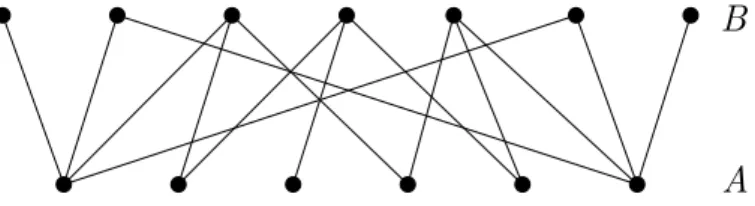
Definition. A bipartite (multi)graph G is a (multi)graph whose vertices can be divided into two disjoint sets Aand B such that all edges ofG connects a vertex in A to a vertex inB, i.e. no two vertices within the same set are adjacent.

A B

Figure 1.4: A bipartite graph

Definition. The complete bipartite graph K_m,n is a bipartite graph with bipartition V =A∪B in which every vertex ofA is adjacent to every vertex ofB, and|A|=m,

|B|=n.

Figure 1.5: The complete bipartite graph K_5,3

1.2 Degrees and the handshake lemma

Definition. In a multigraph G, the degree of a vertex v is the number of edges incident to v, where the loops are counted twice. The degree of v is denoted by deg(v) or deg_G(v).

(15)

v

Figure 1.6: A vertex with degree 7

For example, the vertexv has degree 7 in the multigraph in Figure 1.6.

Remark 1.2. Visually speaking, in a multigraph every edge has two ‘end segments’, associated to the two (not necessarily distinct) endpoints of the edge. In fact, deg(v) is defined to be the number of ‘end segments’ incident to v, that is why loops are counted twice in the above definition.

We note that in a (simple) graph, the degree of a vertex v is simply the number of neighbors of v.

Now we are ready to state and prove the first theorem of every graph theory course.

Theorem 1.3 (Handshake lemma). For any multigraph G, X

v∈V(G)

deg(v) = 2|E(G)|.

That is, the sum of the degrees of all vertices of G is equal to twice the number of edges of G.

Proof. Both sides of the equation count the total number of ‘end segments’ of edges inG (cf. Remark 1.2):

• Since every edge has exactly two end segments, the total number of end segments in G is clearly 2|E(G)|, the right-hand side.

• For any vertex v, the number of end segments incident to v is deg(v), so the total number of end segments is clearly the sum given in the left-hand side of the equation.

Hence the theorem follows.

Corollary 1.4. The sum of the degrees of all vertices is even in any multigraph. In other words, the number of vertices with odd degree is even.

We end this section with a few definitions related to vertex degrees.

Definition. A vertex is called isolated if its degree is 0, i.e. if there are no edges incident to it.

Definition. A multigraph is calledregular if all of its vertices have the same degree.

If the common degree is d in a regular multigraph G, then we also say that G is d-regular.

(16)

1.3 Subgraphs

Definition. LetGbe a multigraph, an edge e∈E(G) and a vertex v ∈V(G) of it.

The multigraph G−e obtained by removing the edge e from Gis defined as V(G−e) := V(G),

E(G−e) := E(G)\ {e}, ψ(G−e) := ψ(G)|E(G−e).

In other words,G−eis the multigraph obtained fromGby deleting the edge efrom the edge set, and the incidences are inherited fromG.

The multigraph G−v obtained by removing the vertex v from G is defined as V(G−e) :=V(G)\ {v},

E(G−e) :=E(G)\ {e∈E(G) :e is incident to v}, ψ(G−e) :=ψ(G)|E(G−v).

In other words, G−v is the multigraph obtained from G by deleting the vertex v (from the vertex set) and the edges incident to v (from the edge set), and the incidences are inherited fromG.

The removal of several edges/vertices can be defined as a natural extension of the above definitons. For a set X ⊆ E(G)∪ V(G), the multigraph obtained by removing the elements of X fromG is denoted by G−X.

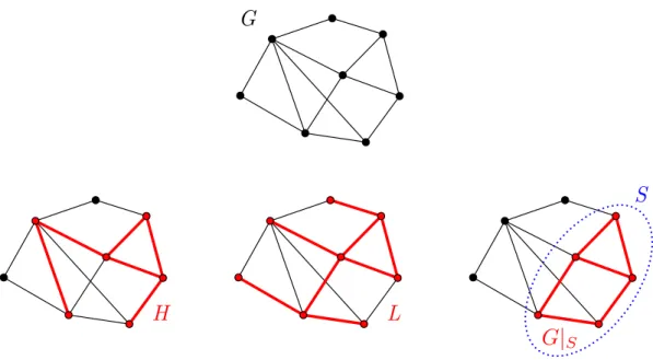
Definition. The (multi)graph H is a sub(multi)graph of the (multi)graph G, ifH can be obtained from G by removing some (or no) edges and vertices. If H is a submultigraph ofG, then we also say that G contains H.

The sub(multi)graph H is a spanning sub(multi)graph of G, if H contains all vertices ofG.

The sub(multi)graph H of G is aninduced sub(multi)graph (on S), if the vertex set ofH is a subsetS ⊆V(G), and H contains exactly those edges of Gwhose both endpoints belong toS. So the induced submultigraphH is determined by the set S, and it is denoted by G|_S.

1.4 Walks, tours, paths, cycles

Definition. A walk in a multigraph G is a sequence

W : (v₀, e₁, v₁, e₂, v₂, e₃, v₃, . . . , v`−1, e_`, v_`),

where v₀, v₁, . . . , v_` ∈ V(G), e₁, . . . , e_` ∈ E(G), and for every e_i (i = 1, . . . , `) its two endvertices are vi−1 and v_i. We say that ` is the length of the walk. ` = 0 is a possibility, ‘(v₀)’ is a path of length 0.

A walk is closed iff v₀ =v_`, otherwise we call it non-closed.

Let V(W) ={v₀, v₁, . . . , v_`}, the vertex set of the walk. Since repeated vertices are not forbidden in the sequence of vertices along a walk,|V(W)| −1 can be much

(17)

L G

H

S

Figure 1.7: A subgraph H, a spanning subgraph L, and an induced subgraph G|_S smaller than the length of W. Let E(W) = {e₁, . . . , e_`}, the edge set of the walk.

Note again, |E(G)| ` is possible.

We emphasize a useful view of walks. We consider it as a dynamic process. The indices are denoting ‘time’. At the beginning (t = 0) we are at vertex v₀ (initial vertex of the walk), from time ito i+ 1 we make a ’step’ from v_i tov_i+1. The walk ends when the clock hits` (end vertex of the walk), we stop inv_`.

On anxy-walk (or xy-path) we mean a walk (or path) with initial vertex x and end vertex y.

Definition. A walk is calledtour iff all ei’s are different, hence|E(W)|is the length of the walk. The notiontrail is also used for a tour.

A walk is called path iff all v_i’s are different, hence |V(W)−1| is the length of the walk.

A walk is called cycle iff ` > 0, and v₀, v₁, . . . , v`−1 are different vertices, but v_` =v₀, furthermore in the case `= 2 we have e₁ 6=e₂.

1.5 Connectivity and trees

This section collects the definitions and fundamental theorems on connectivity as a survey, the proofs are omitted.

Definition. A multigraphGisconnected, if for any two verticesx, y ∈V(G), there exists anxy-walk in G. A multigraph that is not connected is called disconnected.

The following lemma shows that the ‘xy-walk’ can be replaced to ‘xy-path’ in the above definition.

Lemma 1.5. Given a multigraph G, and two vertices x, y ∈ V(G). The following two statements are equivalent:

(18)

(i) There exists an xy-walk in G.

(ii) There exists an xy-path in G.

The following theorem gives the structure of disconnected multigraphs.

Theorem 1.6. Every multigraph G is a vertex-disjoint union of connected multigraphs G₁. . . . , G_k; and this decomposition is unique. (That is, G₁, . . . , G_k are connected induced submultigraphs of G such that there is no edge in G between G_i and G_j for i6=j.)

Definition. The vertex-disjoint connected multigraphs G₁. . . . , G_k in Theorem 1.6 that Gdecomposes into are called the (connected) components of G.

We note that a multigraph is not connected, if and only if it has more than one component.

Now we give some equivalent definitions and the main properties of tree graphs.

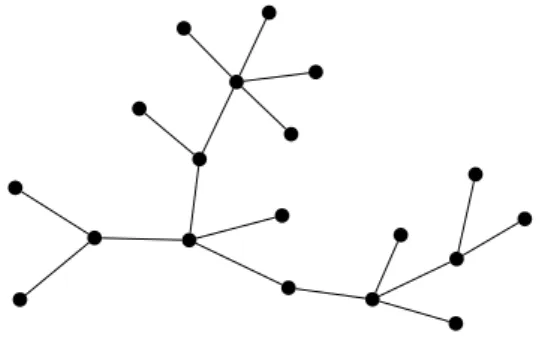
Definition. A graph is a tree, if it is connected and it does not contain a cycle.

Figure 1.8: A tree graph

Theorem 1.7. For any graph G, the following statements are equivalent.

(i) G is a tree.

(ii) G is connected, but the removal of any edge would disconnect it (i.e. G−e is disconnected for all e ∈E(G)).

(iii) For any two vertices x, y ∈V(G), there exists exactly onexy-path inG.

Definition. A vertex with degree 1 in a tree is called a leaf of the tree.

Lemma 1.8. Every tree with at least two vertices has a leaf.

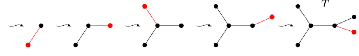
We will need the following operation: Adding a pendant edge to a graphGmeans that we add a new vertexv /∈V(G) to the graph, and connectvby an edge to exactly one old vertex ofG.

Lemma 1.9. (a) For any leaf u of a tree T, the graph T −u is also a tree.

(b) Given a tree T, the tree T^∗ obtained by adding a pendant edge to T is also a tree.

(19)

Theorem 1.10 (Structure theorem of trees). A graph G is a tree if and only if it can be constructed from a single vertex (with no edges) by repeated application of

“adding a pendant edge” operation. In other words, a graph G is a tree if and only if there exists a sequence G₀, G₁, . . . , G_k of graphs such that G₀ is the empty graph on one vertex, G_k =G, and G_i is obtained from Gi−1 by adding a pendant edge, for i= 1, . . . , k. See Figure 1.9.

Figure 1.9: Construction of a treeT by adding pendant edges The structure theorem has an important corollary.

Theorem 1.11. A tree on n vertices has n−1 edges.

We will enumerate spanning trees in Chapter 3.

Definition. Aspanning tree of a multigraph is spanning subgraph which is a tree.

T G

Figure 1.10: A spanning tree Lemma 1.12. Every connected graph has a spanning tree.

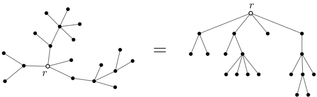
Definition. A rooted tree is a tree with a designated vertex called the root. (For- mally, a rooted tree is a pair (T, r) where T is a tree, and r∈V(T).)

Theorem 1.13.Every rooted tree(T, r)can be drawn like a family tree, as illustrated on the right-hand side of Figure 1.11: The vertices of T are arranged in levels, such that

(i) there is exactly one vertex on the top level, the root r;

(ii) every edge of T connects two vertices on adjacent levels;

(iii) for any non-root vertex u, there is exactly one edge in T that connects u to a vertex on the level just above the level of u.

We note that the level of any vertex v ∈V(T) is uniquely determined. If the length of the unique rv-path in T is `, then v belongs to the (`+ 1)^th level (from top to bottom).

(20)

Figure 1.11: A rooted tree with root r and its family tree-like drawing

(21)

Chapter 2 Graph realizations

Definition. Thedegree sequence of a multigraph is the sequence of degrees of all its vertices, sorted in nonincreasing order. (A sequence d₁, d₂, d₃, . . . is nonincreasing, if d₁ ≥d₂ ≥d₃ ≥. . ..)

Example. The degree sequence of the multigraph in Figure 1.1 is 5,5,4,4,3,2,1.

The main problem of this chapter is to decide that whether there exists a graph whose degree sequence isd or not, for a given sequenced of integers. This problem is called the graph realization problem.

Definition. We say that a finite sequence d of integers can be realized by graph, if there exists a graph G whose degree sequence is d. (If such a graph G exists, we say that G realizes d.)

The realization by multigraph (or by loopless multigraph etc.) is defined analo- gously.

2.1 Realization by multigraphs

The multigraph realization problem is easy.

Proposition 2.1. The nonincreasing sequence d₁, d₂, . . . , d_nof nonnegative integers can be realized by multigraph if and only if the sum d1+d2+· · ·+dn is even.

Proof. Assume first that the sequence d₁, . . . , d_n can be realized by G. By the corollary of handshake lemma (Corollary 1.4), the sum of degrees is even in G, which means that d₁+· · ·+d_n is even.

For the converse, fix a nonincreasing sequence d₁, . . . , d_n of nonnegative integers with the property thatd₁+· · ·+d_nis even. We construct a multigraphGon vertex set {v₁, . . . , v_n} such that deg(v_i) = d_i, for i= 1, . . . , n. The existence of such G will complete the proof. We start with the empty graph on vertex set {v₁, . . . , v_n}, then we addbd_i/2cloops to vertexv_i, fori= 1, . . . , n. At this stage, in the obtained multigraph

deg(v_i) =

(d_i, if d_i is even d_i−1, if d_i is odd

(22)

for alli. This means that for even d_i’s, the corresponding vertexv_i has already had the required degree d_i, but for odd d_i’s, one end segment of an edge is still missing from v_i. This latter issue will be resolved by adding new non-loop edges. Since d₁+d₂+· · ·+d_n is even, thus the number of odd d_i’s is even, and so the number of v_i’s with missing end segment is even. So these v_i’s can be grouped into pairs, and then we can add an edge between every two vertices belonging to the same pair.

In this way all the missing end segments are added, so the obtained multigraph G has degree sequence d₁, . . . , d_n, as required. The construction is illustrated in Figure 2.1.

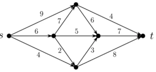
9 7 6 6 3 2 1

Figure 2.1: A multigraph realization of the sequence 9,7,6,6,3,2,1.

.

For completeness, we present the answer to the loopless multigraphs realization problem, but we omit the proof.

Proposition 2.2. The nonincreasing sequenced₁, d₂, . . . , d_n of nonnegative integers can be realized by loopless multigraph if and only if

• d₁+d₂ +· · ·+d_n is even, and

• d₁ ≤d₂+d₃+· · ·+d_n.

2.2 Realization by graphs

Now we discuss the realization problem for graphs. This a much more difficult scenario than the previous ones. Instead of giving an explicit description of the degree sequences, first we present an algorithm to decide whether a sequence can be realized by graph, due to Havel and Hakimi. The algorithm is based on the following key observation.

Lemma 2.3 (Havel–Hakimi). The nonincreasing sequence of nonnegative integers d₁, d₂, . . . , d_n

can be realized by simple graph, if and only ifd1 ≤n−1 and the sequence d₂−1, d₃−1, . . . , d_d₁₊₁−1, d_d₁₊₂, d_d₁₊₃, . . . , d_n

can be realized by simple graph (after reordering the sequence in nonincreasing order).

(23)

Remark 2.4. Note that the second sequence in the lemma can be obtained from the first one by the following operation: Remove the first element, d₁, from the sequence d₁, . . . , d_n, and then in the obtained sequence d₂, . . . , d_n decrease the first d₁ elements by 1. In the future we will denote this operation by HH, so if the first sequence is denoted by d, then the second sequence is HH(d). We apply this operation to nonincreasing sequences only.

Proof of Lemma 2.3. We denote the sequence d₁, . . . , d_n by d, and the second sequence of the lemma by HH(d).

It is easy to see that the conditions are sufficient. Assume that the sequence d₂−1, d₃−1, . . . , d_d₁₊₁−1, d_d₁₊₂, d_d₁₊₃, . . . , d_n

can be realized by a simple graph G. If we add a new vertex v and connect it to those vertices ofG which have degrees d2−1, d3−1, . . . , dd1+1−1, then we obtain a simple graph G⁺ whose degree sequence is d. (The degree of v is d₁ in G⁺, and its neighbors’ degree has been increased by 1, becoming d₂, . . . , d_d₁₊₁.) Hence the sequenced can be indeed realized.

For the converse direction, assume that the sequencedcan be realized by a simple graph G₀. The vertices of G₀ are denoted by v₁, . . . , v_n such that deg(v_i) = d_i, for alli. In a simple graph every degree is at most|V|−1, hence the inequalityd1 ≤n−1 clearly holds. To see that HH(d) can be realized, we will modifyG₀ by adding and deleting edges (without introducing loops or parallel edges), so that in the obtained graphG the vertex degrees are unchanged and the neighbors ofv1 are precisely the verticesv₂, v₃, . . . , v_d₁₊₁. Then the degree sequence of G−v is clearly HH(d), which means that HH(d) can be realized.

Thus in order to complete the proof, it is enough to show that such a modification of G₀ can be done. Recall that deg(v₁) = d₁. If v₁ is adjacent to all the vertices v₂, . . . , v_d₁₊₁, then there is nothing to do, we are done. If this is not the case, we will just see that we can make a degree-preserving modification step onG0 that increases the number of those vertices of {v₂, . . . , v_d₁₊₁} that are adjacent tov₁. And we can repeatedly apply this step until all the vertices v₂, . . . , v_d₁₊₁ become adjacent to v₁, which is our goal.

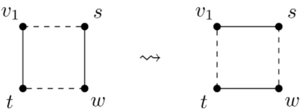
So assume that there is a vertex s∈ {v₂, . . . , v_d₁₊₁} for which v₁s /∈ E(G₀). As deg(v₁) =d₁, there must be a vertext /∈ {v₂, . . . , v_d₁₊₁}inG₀ for whichv₁t∈E(G₀).

Since the sequence d is nonincreasing, deg(s) ≥ deg(t) holds. This, together with the factsv₁s /∈E(G₀) and v₁t ∈E(G₀), implies that inG₀ there exists a neighborw ofs (different from v₁ andt) for whichtw /∈E(G₀). In sum, we have foundv₁, s,w andt, four different vertices ofG0, for whichv1s /∈E(G0),sw∈E(G0),wt /∈E(G0) andtv₁ ∈E(G₀). Now we remove the edgestv₁ and sw fromG₀, and add the edges v₁s and wt, see Figure 2.2. Then we obtain a simple graph G₁ with the same vertex degrees as inG0, in which one more vertex of{v2, . . . , vd1+1}is connected tov1 than inG₀ (since the only changes on the neighborhood ofv₁ are thats entered to it and t left it, where s∈ {v₂, . . . , v_d₁₊₁}, t /∈ {v₂, . . . , v_d₁₊₁}).

This lemma reduces a graph realization problem to an other graph realization problem with smaller input size, so the lemma can be used to solve the problem recursively.

(24)

Figure 2.2: Flip of edges in the proof of Lemma 2.3 .

Theorem 2.5 (Havel–Hakimi algorithm). For a given nonincreasing sequence d of nonnegative integers, the following algorithm decides whether d can be realized by simple graph or not. Moreover, if the answer is yes, a realization graph can be easily constructed, see Remark 2.4.

Havel–Hakimi algorithm (on input sequence d):

• Ifd is a one-element sequence, then it can be realized by simple graph if and only if it is the sequence 0, and the algorithm terminates.

• If the first element ofd is greater than or equal to the number of elements of d, then d cannot be realized and the algorithm terminates.

• Otherwise, calculate HH(d).

• If the sequence HH(d) contains a negative number, then dcannot be realized and the algorithm terminates.

• Otherwise, reorder the sequence HH(d) in nonincreasing order, and invoke this algorithm recursively on input sequence HH(d). The obtained answer is the answer to the initial question (on input d).

The Havel–Hakimi-algorithm is just the repeated application of Lemma 2.3. It can be best understood through examples.

Example. As a first example, we decide, using the Havel–Hakimi-algorithm, if the sequence 7,4,3,3,3,3,2,1,0 can be realized by simple graph:

7,4,3,3,3,3,2,1,0 can be realized m

3,2,2,2,2,1,0,0 can be realized m

1,1,1,2,1,0,0 can be realized

|| (reorder) 2,1,1,1,1,0,0 can be realized

m

0,0,1,1,0,0 can be realized

|| (reorder)

(25)

1,1,0,0,0,0 can be realized m

0,0,0,0,0 can be realized.

Since the sequence 0,0,0,0,0 can be trivially realized by the empty graph on five vertices, hence the initial sequence 7,4,3,3,3,3,2,1,0 can realized, too. (We note that Theorem 2.5 defines the algorithm to run until it reaches to the one-element sequence 0. But, of course, we can stop at any point when we see that the actual sequence can be realized. And this is the case for all-0 sequences, for example.) Remark 2.6. It is important to note that in case of positive answer, the Havel–

Hakimi-algorithm not only proves the existence of a graph that realizes the input sequence, but such a graph can be easily read off from the sequences that appears during the algorithm’s run. The point is that if we know a realization graph G for the sequence HH(d), then a realization graph for the sequence d can be easily constructed from G: This is the first (easy) part of the proof of Lemma 2.3 (add a new vertex to G and connect it to the vertices with decreased degrees). So we can go through the sequences appearing during the algorithm’s run in reverse order, and starting from the trivial realization of the final sequence, reach to a realization of the input sequence of the algorithm. In the example above, from the (empty graph) realization of 0,0,0,0,0, we can obtain a realization for 1,1,0,0,0,0 by the above method. And from the realization of 1,1,0,0,0,0, we can obtain a realization for 2,1,1,1,1,0,0, and so on.

Example. As a second example, we decide if the sequence 8,8,6,6,6,5,3,2,2 can be realized by simple graph:

8,8,6,6,6,5,3,2,2 can be realized m

7,5,5,5,4,2,1,1 can be realized m

4,4,4,3,1,0,0 can be realized m

3,3,2,0,0,0 can be realized m

2,1,−1,0,0 can be realized.

Clearly, the sequence 2,1,−1,0,0 cannot be realized by graph as it contains a negative number, hence the inital sequence cannot be realized neither.

There is an explicit description of degree sequences of simple graphs, due to Erd˝os and Gallai. We omit the proof.

Theorem 2.7 (Erd˝os-Gallai). The nonincreasing sequence d₁, d₂, . . . , d_n of nonnegative integers can be realized by simple graph if and only if

• d₁+· · ·+d_n is even, and

(26)

• for all k∈ {1, . . . , n},

k

X

i=1

d_i ≤k(k−1) +

n

X

i=k+1

min(d_i, k).

2.3 Realization by trees

We end this chapter with the realization problem on trees.

Proposition 2.8. For n ≥2, the nonincreasing sequence d₁, . . . , d_n of nonnegative integers can be realized by tree if and only ifPn

i=1d_i = 2(n−1) holds andd_i >0 for all i.

Proof. If the sequence can be realized by a tree T, then by the handshake lemma,

n

X

i=1

d_i = 2|E(T)|= 2(n−1),

using also the fact that a tree on n vertices has n−1 edges. And a tree (on at least two vertices) cannot have isolated vertex, so d_i >0 holds for all i, too.

Conversely, the statement “if Pn

i=1d_i = 2(n −1), and d_i > 0 for all i, then the sequence d₁, . . . , d_n can be realized by tree” is proved by induction on n. The base case n = 2 can be verified easily. (1,1 is the only sequence that satisfies the conditions, which can be clearly realized.) For the inductive step, assume that the sequence d₁, . . . , d_n satisfies the conditions. Then observe that the average of the numbersd₁, . . . , d_n is between 1 and 2, because

1 n

n

X

i=1

d_i = 1

n ·2(n−1) = 2− 1 n

andn≥2. This implies thatd₁, the largest element, must be at least 2, andd_n, the smallest element, must be at most 1. Since d_n >0 by the conditions, we conclude thatdn = 1. Hence the (n−1)-element sequenced1−1, d2, d3, . . . , dn−1 satisfies the conditions of the theorem, as d₁ −1 > 0 and the sum of its elements is 2(n−2).

So, by the induction hypothesis, this sequence can be realized by a tree T⁰ onn−1 vertices. If we add a new vertex toT⁰ and join it to the vertex of degreed1−1, then we obtain a tree T that realizes the sequence d₁, . . . , d_n, completing the proof.

Remark 2.9. The inductive part of the proof can be easily algorithmized to construct a tree that realizes a given nonincreasing sequence d₁, . . . , d_n satisfying the conditions of Proposition 2.8: Invoke the algorithm recursively on the sequence d₁−1, d₂, d₃, . . . , dn−1 (after reordering it in nonincreasing order), and then add a new vertex to the output treeT⁰ and connect it to the vertex of degreed₁−1. The recursion terminates when the number of vertices reaches 2.

In the next chapter we will prove even more on this subject, Corollary 3.7 gives the exact number of trees realizing a given sequence.

(27)

Chapter 3 Enumeration of spanning trees

This chapter deals with the number of spanning trees of a given graph. (Recall the definion of spanning trees from Chapter 1.) In this subject, two spanning trees are considered the same if and only if they have the same edge set.

3.1 Spanning trees of complete graphs

The following classical enumeration result gives the number of spanning trees in complete graphs, cf. Figure 3.1.

1 2

3 4

1 2

3 4

1 2

3 4

1 2

3 4

1 2

3 4

1 2

3 4

1 2

3 4

1 2

3 4

1 2

3 4

1 2

3 4

1 2

3 4

1 2

3 4

1 2

3 4

1 2

3 4

1 2

3 4

1 2

3 4

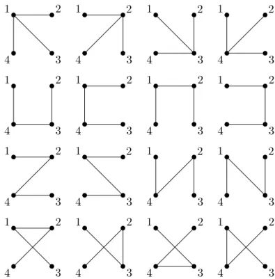
Figure 3.1: The spanning trees of K₄

Theorem 3.1 (Cayley). The number of spanning trees of the n-vertex complete graph is nⁿ⁻².

(28)

We will prove Cayley’s theorem soon by giving a bijection between the set of spanning trees of K_n and the set of sequences of n−2 elements of{1,2, . . . , n}.

But first we look at the spanning trees of the complete graphK_n from a different viewpoint. As every two vertices are adjacent inK_n, a spanning tree ofK_n is just a tree on the vertex set ofK_n. We can assume thatV(K_n) ={1, . . . , n}, so a spanning tree of K_n is just a tree on vertex set {1, . . . , n}. We will use this viewpoint if we do not want to deal with the underlying graph K_n, and we even use a different terminology then.

Definition. A labeled tree on n vertices is a tree on vertex set {1, . . . , n}. In order to be consistent with the spanning tree enumeration problem, the labeled trees T₁ andT₂ (on n vertices) are considered the same if and only if exactly the same pairs of vertices are adjacent in T₁ as in T₂.

Remark 3.2. The name ‘labeled tree’ reflects the fact that we usually think of vertex i(where i∈ {1, . . . , n}) as a node labeled with the number i, see Figure 3.2.

Hence sometimes we refer to vertex i as vertex withlabel i, too.

1

9 11 5

12

3 2 6

7

4 10

8

Figure 3.2: A labeled tree on 12 vertices

With this terminology, Cayley’s theorem can be formulated as follows.

Theorem 3.3 (Cayley). The number of labeled trees on n vertices is nⁿ⁻².

As promised, we encode now the labeled trees on n vertices into sequences of n−2 elements of{1,2, . . . , n}, due to Pr¨ufer.

Definition (Pr¨ufer encoding). Let T be a labeled tree on n vertices, where n≥ 2.

The Pr¨ufer code of T, denoted by Pr(T), is a sequence defined by the following procedure:

• Find the leaf of T which has the smallest label among the leaves of T; and let us denote this leaf by u₁. Add the label of u₁’s (unique) neighbor to Pr(T) as first element, and then remove the leaf u₁ from T.

• Repeat the previous step on the obtained labeled treeT−u₁(cf. Lemma 1.9.a):

Find the leaf of T −u1 with smallest label, say u2, and add the label of u2’s neighbor to Pr(T) as second element, then remove the leaf u₂.

(29)

• And so on, in the k^th step, we define the k^th element of Pr(T) to be the label of the neighbor of the smallest-labeled leaf in T^(k−1), where T^(k−1) is the tree obtained from T after removing the vertices u₁, . . . , u_k−1 in the former steps;

then remove the smallest-labeled leaf u_k from this tree.

• The process terminates aftern−2 step, i.e. when the number of vertices in the actual tree is 2. (At that point the modification step is not executed further.) We note that it is obvious from the above description that Pr(T) has n−2 elements and its elements are from the set{1, . . . , n}.

Example. For example, the Pr¨ufer code of the labeled tree in Figure 3.2 is 12,8,8,12,3,6,8,1,1,6.

Cayley’s theorem (Theorem 3.3) is directly implied by the following lemma.

Lemma 3.4 (Pr¨ufer). Let n be a fixed integer at least 2. The mapping T 7→Pr(T) is a bijection from the set of labeled trees on n vertices to the set of (n−2)-element sequences of {1, . . . , n}.

Proof. We will prove a slightly more general statement. For any finite set V ⊂ N, we can consider labeled trees onV, by extending the original definition to arbitrary vertex (label) set: A labeled tree on V is just a tree on vertex set V (interpreting its vertices as labels). The definition of Pr¨ufer encoding also applies to labeled trees on vertex set V without any modification. We will prove the following statement by induction on n: “For any fixed finite set V ⊂ N with n ≥ 2 elements, the mapping T 7→ Pr(T) is a bijection from the set of labeled trees on V to the set of (n−2)-element sequences of V.”

The case |V| = 2 is obvious, so we can assume that |V| > 2. We have to prove that for any (n−2)-element sequence s of V, there exists a unique labeled tree on V whose Pr¨ufer code is s. To this end, fix an arbitrary (n −2)-element sequence s = (s₁, . . . , sn−2) of V, and assume that T_s is a labeled tree on V for which Pr(T_s) = s.

Observe first that vertex v of the labeled tree T is a leaf if and only if v is not contained in the sequence Pr(T). This is because if v is a leaf, then we never remove the neighbor of v during the Prüfer encoding (and hence v is never added to the Prüfer code), because we always remove a leaf, and the neighbor of v can be also a leaf only if there are no other vertices in the tree (when the process already terminates). And if v is not a leaf, then during the Prüfer enconding the degree of v must decrease at some point (because v will become a leaf eventually, no matter whether v will be deleted from the tree or v is one of the two surviving vertices);

and when the degree of a vertex decreases then the vertex is added to the Pr¨ufer code.

This means that we know an important information on the tree T_s (with Pr¨ufer codes): The leaves ofT_smust be exactly those vertices fromV that are not contained in the sequences. (At least two such vertices exist, because while V has n vertices, shas only n−2 elements.) Let u denote the smallest of the leaf vertices. We know that in the first step of the Pr¨ufer encoding of T_s, the removed leaf is u and it was

(30)

connected to vertexs₁. And then the obtained treeT_s−u, a labeled tree on vertex set V \ {u}, was Pr¨ufer-encoded into (s₂, . . . , sn−2), a sequence of n −3 elements of V \ {u}. By the induction hypothesis, there exists exactly one labeled tree on V \ {u}, say T⁰, whose Pr¨ufer code is (s₂, . . . , sn−2). So T_s−u must be this tree T⁰, and hence T_s can only be the tree obtained from T⁰ by adding vertex u and connecting it tos₁.

It is straightforward to verify that the Prüfer code of this unique tree T_s is indeed s. (We have to check that after connecting u to vertex s₁ of T⁰, u indeed becomes the smallest leaf (label) in the obtained tree T_s – this is required to verify thatuis the first removed vertex in the Prüfer encoding ofT_s, as expected. This can be easily done by determining the leaves of T⁰ from its Prüfer code (s₂, . . . , sn−2), as discussed in the third paragraph of this proof.)

The above proof is a bit terse, an example will shed more light on the recursive reconstruction of the labeled tree from its Pr¨ufer code.

Example (The inverse of Pr¨ufer encoding). As an example, we will find the unique labeled treeT (on 9 vertices) whose Pr¨ufer code is the following 7-element sequence of {1, . . . ,9}:

4,1,4,2,4,9,2.

For shortness, vertexv and label v will be identified (like in the formal definition of labeled trees). And T⁽ⁱ⁾ will denote the tree obtained from T after processing the first i steps (vertex removals) of the Pr¨ufer encoding of T.

1. The leaves of T are exactly those elements of V(T) = {1, . . . ,9} which are not contained in the sequence 4,1,4,2,4,9,2; so the leaves of T are precisely 3,5,6,7,8. The smallest of them, vertex ‘3’, was removed in the first step of the Pr¨ufer endoding, and it was adjacent to the first element of the sequence, vertex ‘4’. So we conclude that 34 is an edge of T. (Here 34 denotes an edge connecting the vertices ‘3’ and ‘4’.)

2. The leaves of T⁽¹⁾, the tree obtained from T after removing vertex ‘3’, are exactly those elements of V(T⁽¹⁾) = {1, . . . ,9} \ {3} which are not contained in the truncated sequence 1,4,2,4,9,2; i.e. the leaves of T⁽¹⁾ are precisely 5,6,7,8. This means that in the second step of the Pr¨ufer encoding, the smallest of them, vertex ‘5’ was removed from T⁽¹⁾, and it was adjacent to ‘1’, so 51 is also an edge of T.

3. In the third step of the Pr¨ufer encoding ofT, the removed leaf ofT⁽²⁾ was ‘1’, the smallest element of V(T⁽²⁾) ={1, . . . ,9} \ {3,5}which is not contained in the sequence 4,2,4,9,2. The neighbor of the removed leaf ‘1’ is ‘4’, so 14 is an edge of T.

4-7. And so on, we can figure out in a similar way that the vertices ‘6’, ‘7’, ‘4’

and ‘8’ were removed in the 4^th, 5^th, 6^th and 7^th steps of the Pr¨ufer encoding, respectively. The second row of Table 3.1 contains the sequence of removed vertices; the vertex in thei^th position was removed in thei^thstep. (Remark 3.5 will discuss a mechanical way to fill this table.) The neighbors can be read off from the Pr¨ufer code, so we found the edges 62, 74, 49 and 82 in T.

(31)

Pr¨ufer code 4 1 4 2 4 9 2 removed leaf 3 5 1 6 7 4 8 Table 3.1: The steps of reconstruction

8. Finally, we know that after removing the seven vertices determined above, we end up with a 2-vertex tree, i.e. the two remaining vertices, ‘2’ and ‘9’ are connected by edge, and hence 29 is also an edge inT. Now we have determined all edges of T: they are 34,51,41,62,74,49,82 and 29, so we conclude that T is the labeled tree on Figure 3.3.

1 9

5

3 6

2 7

4

8 Figure 3.3: The solution to the exercise

We note that the reasonings in steps 1-8 do not showwhy the determined edges form a tree. That follows from the inductive argument of the proof of Lemma 3.4.

Remark 3.5. It is easy to see that both the Pr¨ufer encoding and its inverse can be implemented efficiently on computer. For example, the construction of Table 3.1, the heart of the above inversion algorithm, can be summarized as follows. The elements of the second row are filled from left to right, such that the i^th element of the second row is the smallest number in{1, . . . , n}which occurs neither among the first i−1 elements of the second row nor among the last n−i+ 1 elements of the first row.

The observation made in the proof of Lemma 3.4 can be extended, which can be used to count the number of trees with a given degree sequence.

Lemma 3.6. For an arbitrary labeled tree T, any vertex v of T occurs exactly deg(v)−1 times in the Pr¨ufer code of T.

Proof. The proof is left to the reader as an exercise.

Corollary 3.7. For n ≥ 2, let d₁, . . . , d_n be a sequence of integers that can be realized by tree, that is, by Proposition 2.8, a sequence for whichPn

i=1d_i = 2(n−1) holds and d_i > 0 for all i. Then the number of those (labeled) trees on vertex set {1, . . . , n} in which deg(i) =d_i holds fori= 1, . . . , n, is

(n−2)!

(d₁−1)!(d₂−1)!. . .(d_n−1)!.

(32)

Proof. Since the Pr¨ufer encoding encodes trees on vertex set {1, . . . , n}into (n−2)- element sequences of {1, . . . , n} bijectively, it is enough to count those (n − 2)- element sequences of{1, . . . , n}which belong to trees satisfying the degree conditions deg(i) =d_i. Fortunately, the degrees of vertices can be easily read off from the Pr¨ufer code by Lemma 3.6: We have to count those (n −2)-element sequences in which the elementi occurs exactly d_i−1 times, for all i∈ {1, . . . , n}. (This makes sense becaused_i−1≥0 for alli, andPn

i=1(d_i−1) =n−2, as implied by the conditions.) These sequences are exactly the permutations of the (n−2)-element multiset

{1,1, . . . ,1

| {z }

d1−1 times

,2,2, . . . ,2

| {z }

d2−1 times

, . . . , n, n, . . . , n

| {z }

dn−1 times

}.

The well-known formula on the number of permutations of a multiset yields the answer

(n−2)!

(d1−1)!(d2−1)!. . .(dn−1)!

to the enumeration problem.

3.2 Spanning trees of arbitrary graphs

Without a proof, we present a famous theorem that expresses the number of spanning trees of a given graph as a determinant. What makes it applicable in practice is that determinants can be calculated effectively by computer. In addition, the theorem has many theoretical consequences, too – as an application, we deduce Cayley’s theorem from it.

Theorem 3.8(Kirchhoff’s matrix tree theorem).A graphGon vertex set{v₁, . . . , v_n} is given. Then×n matrix L_G is defined as follows. (L_G)_ij, the element lying in the i^th row and the j^th column of L_G, is







deg_G(v_i), if i=j

0, if i6=j, and v_i is not adjacent to v_j

−1, if i6=j, and v_i is adjacent to v_j.

In words, the diagonal elements of LG are the degrees of vertices, and every off- diagonal element is equal to (−1) times the number of edges between the two corresponding vertices. And let L⁽⁻ⁱ⁾_G denote the (n−1)×(n−1) matrix obtained from L_G by deleting the i^th row and the i^th column of it.

Then the determinant of L⁽⁻ⁱ⁾_G counts the number of spanning trees of G, for any fixed i∈ {1, . . . , n}.

Example (Cayley’s theorem as a corollary of the matrix tree theorem). As an application, we deduce the number of spanning trees of the complete graph Kn

again, now using the matrix tree theorem.

(33)

Following the notations of the theorem, we clearly have

L_K_n =







n−1 −1 −1 · · · −1

−1 n−1 −1 · · · −1

−1 −1 n−1 · · · −1 ... ... ... . .. ...

−1 −1 −1 · · · n−1







n×n

,

and hence

L⁽⁻¹⁾_K

n =







n−1 −1 · · · −1

−1 n−1 · · · −1 ... ... . .. ...

−1 −1 · · · n−1







(n−1)×(n−1)

.

By the matrix tree theorem, the number of spanning trees ofK_nis equal to det(L⁽⁻¹⁾_K

n ), so we have to calculate this determinant.

det(L⁽⁻¹⁾_K_n ) =

n−1 −1 · · · −1

−1 n−1 · · · −1 ... ... . .. ...

−1 −1 · · · n−1

(n−1)×(n−1)

=

1 1 · · · 1

−1 n−1 · · · −1 ... ... . .. ...

−1 −1 · · · n−1

(n−1)×(n−1)

=

1 1 · · · 1 0 n · · · 0 ... ... . .. ...

0 0 · · · n

(n−1)×(n−1)

=nⁿ⁻².

The second determinant was obtained from the first one by adding the 2^nd,3^rd, . . . , (n −1)^th rows to the 1^st row, and then the third determinant was obtained from the second one by adding the 1^st row to the 2^nd,3^rd, . . . ,(n−1)^th rows. (These operations do not change the value of the determinant.) Finally, we used the linear algebra fact that the determinant of an upper triangular matrix is equal to the product of the elements in its main diagonal.

(34)

Chapter 4 Network flow problems

4.1 Network Flow Problems

The mathematical abstraction of networks is particularly useful. One can model a water pipe network or currents in an electrical network (and many other real life problems) using network flows, and it is also a valuable tool for studying certain combinatorial optimization problems. In this chapter we will present the basics of the area and some applications.

First a notation. Given a directed multigraph G= (V, E) and any vertexv ∈V, we letE⁺(v) denote the set of edges leaving v, and E⁻(v) denotes the set of edges entering v. Hence, the outdegree of v is deg⁺(v) =|E⁺(v)| and the indegree of v is deg⁻(v) = |E⁻(v)|.

Definition. LetG=G(V, E) be a directed multigraph with two distinguished vertices, s and t such that s 6= t. Let c : E −→ R⁺ be the function. In a network N(G, s, t, c) with underlying directed braph G we call s the source and t the sink, and cis the capacity function of the edges of G.

Given a function f :E −→ R we say that f is a feasible flow in N if the following conditions hold:

Capacity constraints : for every e∈E(G) we have 0≤f(e)≤c(e).

Conservation constraints: for every v ∈V − {s, t} we have X

e∈E⁺(v)

f(e) = X

e∈E⁻(v)

f(e)

The value of a feasible flowfis defined to beval(f) =P

e∈E⁺(s)f(e)−P

e∈E⁻(s)f(e).

Given subsetsS ⊂V, s∈S andT ⊂V, t∈T such that S∪T =V and S∩T =∅ is called an [S, T]-cut (or source/sink-cut). The edge set of the cut is E({S, T}) that contains exactly those edges with one endpoint in S and the other endpoint in T.

The edge setE([S, T]) can naturally be divided into two disjoint subsets: −→ E =−→

ST

(35)

contains the edges that point from S towardsT, while ←− E =−→

T S contains the edges with tail inT and head inS.

Given an [S, T]-cut and a feasible flow f in a network N the value of the cut is defined to beval(S, T) =P

e∈−→

ST f(e)−P

e∈−→

T Sf(e).

Our goal is to find a feasible flow having maximum value. The following helps in achieving this goal.

Lemma 4.1.

val(S, T) =val(f).

Proof. By induction on the cardinality of S. It clearly holds when |S| = 1, that is, whenS ={s}.One only have to verify that the value does not change when placing an arbitrary vertex other than t fromT toS.

Definition. The capacity of an [S, T]-cut is the total capacity of edges in−→

ST , that is, we sum up the capacities of edges with tail inS and head inT. It is denoted by c(S, T).

Easy to see:

max

f is a flowval(f)≤ min

[S,T]−cutc(S, T).

The theorem below shows that much more is true (we will prove this later).

Theorem 4.2. [Maximum Flow–Minimum Cut theorem] Let N(G, s, t, c) be a network. Then

max

f is a flowval(f) = min

[S,T]−cutc(S, T).

We will refer to this result as the MFMC theorem.

Remark 4.3. When the two sides equal for some feasible flow f and an [S, T]-cut as in the MFMC theorem, then the edges fromS toT “work” at full capacity, while f is zero on every edge that goes from T to S.

Definition. Let P be an undirected s−t path, i.e., a path which leads from s tot in the graph we obtain from G by making its edges undirected. Assume that f is a feasible flow in N(−→

G , s, t, c). We divide the edges of P into two disjoint subsets, E^{f wd}(P) andE^bwd(P).The edgee∈E(−→

G)∩E(P) belongs toE^{f wd}(P) if we traverse e according to its orientation when going from s to t along P. Otherwise, if we traverseeagainst its orientation, thene∈E^bwd(P).We say thatP is an augmenting path with respect to flow f if

- f(e)< c(e) for every e∈E^{f wd}(P) and

(36)

- f(e)>0 for every e∈E^bwd(P).

Let

δ^{f wd} := min{c(e)−f(e) :e∈E^{f wd}(P)}, δ^bwd := min{f(e) :e∈E^bwd(P)}, and

δ := min{δ^{f wd}, δ^bwd}.

We have the following lemma.

Lemma 4.4. Let f be a feasible flow in the network N(G, s, t, c). If N has an augmenting path P with respect to f, then the value of f is not optimal, one can find another feasible flow f⁰ in N for which

val(f) +δ=val(f⁰), where δ is as defined above.

Proof. The proof essentially consists of two observations. The first one is that f⁰ is a feasible flow using the definition of δ, neither the capacity constraints, nor the conservations constraints are violated. Secondly, if we take an arbitrary [S, T]-cut, its value increases precisely by δ. These observations prove what was desired.

One might think that the following scenario is possible: there exists some network N(G, s, t, c) and a feasible flow f in N such that f is not optimal, but there is no augmenting path inN with respect tof. Fortunately, this is not the case.

Theorem 4.5. Letf be a flow in networkN(G, s, t, c).The following are equivalent:

1. f is a maximum flow

2. there exists an [S, T]-cut, for which val(f) = c(S, T)

3. there is no augmenting path in N(G, s, t, c) with respect to f

Observe that the MFMC theorem is implied by Theorem 4.5. In order to prove Theorem 4.5 we need a new notion and a lemma.

Definition. Let P be a path, with one endpoint being s, in the graph we obtain fromGby making its edges undirected. The edge set ofP is divided into the disjoint sets E^{f wd}(P) and E^bwd(P), as before. We say that P is a partial augmenting path inN(G, s, t, c) if the followings hold: (i) for every e∈E^{f wd}(P) we have f(e)< c(e) and (ii) for everye∈E^bwd(P) we have f(e)>0.

Lemma 4.6. Let f be a maximum flow in network N(G, s, t, c). Let S be the set of those vertices that can be reached from s by some partial augmenting path. Finally, let T =V −S. Then [S, T] is a minimum cut with capacity c(S, T) = val(f).