Early childhood and primary education efficiency in Europe: a data envelopment analysis approach
BOGDAN DIMA Professor
East European Center for Research in Economics and Business, West University of Timişoara, Romania
Email: bogdan.dima@e-uvt.ro BALÁZS KOTOSZ
Adjunct Professor
IÉSEG School of Management, France
Email: b.kotosz@ieseg.fr
ŞTEFANA MARIA DIMA Senior Researcher
East European Center for Research in Economics and Business, West University of Timişoara, Romania
Email: stefana.dima@e-uvt.ro
This study explores the use of data envelopment analysis with bias correction of technical efficiency scores to measure ‘efficiency’ in early childhood and primary education. It also advances a potential framework derived from the ‘human capital paradigm’ to support the selection of inputs and outputs in efficiency assessment. Finally, it illustrates some specific features of early childhood and primary education in Europe (as well as the United States and Japan as referential countries) and provides empirical evidence on the heterogeneity of ‘education technologies’ and their perfor- mances among these countries. It is found that Nordic countries have the highest output-based technical efficiency.
KEYWORDS: early childhood and primary education, DEA, European countries
C
urrently, more and more studies deal with the application of DEA (data envelopment analysis) in the measurement of efficiency in secondary (Soteriou et al.[1998]) or higher education (Abbott–Doucouliagos [2003], Johnes [2006], Glass et al. [2006], Thanassoulis et al. [2010], Nazarko–Šaparauskas [2014]).
These studies address several issues related to the prospect of implementing an efficiency analysis at the level of education units. However, such studies usually suffer from several limitations that bias their results and interpretation. First, these
studies do not state comprehensively that DEA is applicable for measuring efficiency in the education sector. More exactly, they do not present arguments for the idea that the usual economic assumptions considered in the general efficiency analysis might be adopted here as well. Second, deficiency of the theoretical grounds frequently occurs when defining the explicit sense of the term ‘efficiency’ in education.
The pure economic approach of this concept cannot be considered ‘as it is’, when the assessment of educational outputs is considered. Instead, a more comprehensive framework must be advanced to integrate all the monetary and non-monetary out- comes of education. In the absence of such a framework, the assortment of input and output variables designed to capture the key dimensions of education can take place only on ad-hoc bases. Third, only few studies go beyond the standard DEA analysis by considering more complex DEA methods (for instance, robust DEA aiming to correct for data biases, two- and three-stage DEA allowing the introduction of envi- ronmental variables, and so on). Fourth, these studies generally have little to say about the specific ‘education technology’. The assumption of ‘decreasing returns to scale’, which is standard for economic studies, may not be appropriate in the educa- tion sector, and other choices for the relevant technology should be justified.
Fifth, there are only a few international comparative analyses concerning the primary stages of education (Sutherland et al. [2007], Miningou–Vierstraete [2013]), and such studies highlight, to a lesser extent, the distinctive features of primary edu- cation as compared with the next education stages.
Our study’s contributions are two-fold. On the one hand, we discuss some merits (and limits) of DEA in valuing the efficiency of educational processes.
On the other hand, we illustrate the possibilities of applying this approach, based on a theoretical framework derived from the human capital paradigm, to assess early childhood and primary education in Europe (as well as the United States and Japan as referential countries). Our argument is based on the idea that the human capital model can provide a solid theoretical framework to support both the selection of the corresponding educational descriptors to be included in the efficiency analysis and the discrimination of their relative importance.
Hence, Section 1 describes the methodological background of DEA and the possibility for it to capture some specific features of early education stages. Section 2 provides some details on international data, while Section 3 reports the empirical results. The last section provides the conclusions.
1. Methodological background
This section describes the employed methodological framework. First, a sum- mary description of DEA, as the main involved technique, is presented. Second, the human capital paradigm of education is discussed. Third, some specific features for early education cycle are highlighted.
1.1. Data envelopment analysis
Developed as linear programming estimators by Charnes–Cooper–Rhodes [1978], DEA provides an approach to the issue of efficiency (and effectiveness) of societal structures and activities. As Bogetoft and Otto ([2011] p. 81.) notes:
‘A short definition of DEA is that it provides a mathematical programming method of estimating best practice production frontiers and evaluating the relative efficiency of different entities.’ Its usefulness resides in this framework capability of analysing a multi-process activity. Each of the component processes involves a series of input vectors and generates intermediary/final outcomes. Being complementary, each of these processes is characterised by specific sets of (possible) inter-related technolo- gies. Hence, DEA allows a systematic approach to complex entities, if their activity can be described in terms of (economic) efficiency.
In applying DEA, there is a specific approach to the concept of efficiency.
According to Daraio–Simar ([2007] p. 14.), this concept is viewed ‘as a distance between the quantity of input and output, and the quantity of input and output that defines a frontier, the best possible frontier for a firm in its cluster (industry)’.
Thus, it appears that efficiency is a distinctive (yet related) concept to productivity, as this can be defined (in a global sense) as the ratio between outputs (outcomes of an activity that has an economic dimension) and inputs (all the efforts associated with such an activity). Farrell [1957] identifies three types of efficiency:
a) technical, b) allocative (labelled by Farrell as ‘price efficiency’), and c) economic efficiency (or, in Farrell’s terminology, overall efficiency). The first type of efficiency refers to the ability of a DMU (decision-making unit) to obtain the maximum feasible output from a given bundle of inputs (if we consider an output-oriented technical effi- ciency) or, alternatively, to involve a minimum feasible amount of inputs to produce a given level of output (if an input-oriented technical efficiency is considered). Alloca- tive efficiency refers to the ability of a technically efficient DMU to use inputs in a way that minimises production costs given input prices. Finally, economic efficiency is the combined outcome of both the technical and allocative forms of efficiency.
A key issue in assessing efficiency is that such efficiency measures imply the ex- istence of a known production function (and, implicitly, a known technological set;
Manyeki–Kotosz [2019]). If such function is not known, then the relative estimates of efficiency must be derived from available data samples. Usually, two approaches can be applied to fulfil this task: the parametric or SFA (stochastic frontier production approach) and the nonparametric or DEA approach. Due to its nonparametric nature and in contrast to SFA, DEA does not impose any assumptions on the functional form of the frontier and/or the distribution of the error term. Still, an important disadvantage of DEA is that all deviations from the frontier reflect inefficiency. Hence, bias correc- tion methods are necessary to compensate for the potential noise associated with data measurement errors, incomplete data, ‘structural breaks’ in data, or other factors.
Key concepts
A key concept in a DEA framework is the ‘Farrell efficiency’ (Farrell [1957]).
As Bogetoft and Otto ([2011] p. 15.) explains: ‘The idea of the Farrell measures is to focus on proportional changes – the same percentage reducing in all inputs or the same percentage increase in all outputs… The Farrell input efficiency measures how much we can proportionally reduce the input and still produce the same output…
In the same way we can define the output efficiency as the largest factor that we can multiply on the output and still have a possible production for given input.’
Formally, input-based Farrell efficiency of a set of inputs x and outputs y relative to a technology set T (i.e. input-output combinations that are presumed to be feasible in a given context) can be defined as:
E min
E 0
Ex y,
T
. /1/It is the maximal proportional possible reduction of all inputs x that allows the production of the same level of y.
In a similar way, output-based Farrell efficiency might be defined as:
F max
F 0
x Fy,
T
. /2/In other words, this is the maximal proportional expansion of all outputs y that can be reached without modifying the used levels of inputs x.
However, the idea of proportionally adjusting by increasing/decreasing all out- puts/inputs with the same factor seems to be less plausible for real-life cases. Hence, other measures have been proposed for the efficiency assessment. Among these al- ternative measures, an interesting approach is provided by ‘directional distance func- tions’. The purpose here is ‘to determine improvements in a given direction
d
m and to measure the distance to the frontier in such d-units’ (Bogetoft–Otto [2011] p. 32.).
Thus, the directional distance functions can be viewed as an excess function, e (with
d d
x,
y
mX
n ):ee x y T d
, ; ,
: max
e
x ed x, y ed y
T
. /3/There is a straightforward interpretation of ‘excess’ e: ‘the input bundle d has been used in x in excess of what is necessary to produce y’ (Bogetoft–
Otto [2011] p. 32.). Thus, ‘a large excess reflects a large (absolute) slack and a con- siderable amount of inefficiency’ (idem).
Nevertheless, in a broader sense, the direction distance function approach examines ‘whether it is possible to use fewer inputs and produce more outputs’
(Bogetoft–Otto [2011] p. 33.).
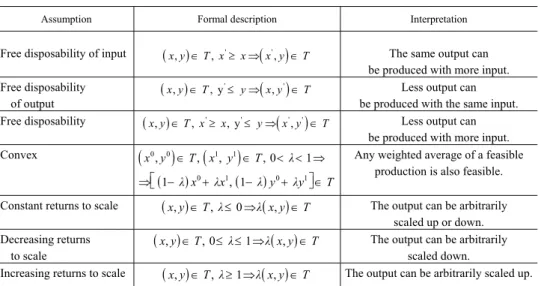
Technology assumptions
Moreover, several assumptions can be made regarding the technological set T as shown in Table 1 (for a more detailed discussion, see Bogetoft–Otto [2011]
pp. 74–77. or Zalai [2000]).
Table 1 Assumptions on the technological set
Assumption Formal description Interpretation
Free disposability of input x y, T x, ' x x y', T The same output can be produced with more input.
Free disposability
of output x y, T, y' yx y, 'T Less output can be produced with the same input.
Free disposability x y, T x, ' x, y' yx y', 'T Less output can be produced with more input.
Convex
0 0 1 1
0 1 0 1
, , , , 0 1
1 , 1
x y T x y T λ
λ x λx λ y λy T
Any weighted average of a feasible production is also feasible.
Constant returns to scale x y, T,λ 0 λx y, T The output can be arbitrarily scaled up or down.
Decreasing returns to scale
x y, T, 0 λ 1 λx y, T The output can be arbitrarily scaled down.
Increasing returns to scale x y, T,λ 1 λx y, T The output can be arbitrarily scaled up.
Note. x and y denote inputs and outputs respectively, and T is a technology set.
Additionally, a technology that exhibits increasing, constant, or decreasing re- turns to scale in different regions can be labelled as one of ‘variable returns to scale’.
All these assumptions can be considered with both input- and output-oriented efficiency and can lead to distinctive specifications of the involved optimisation problems. The R language package ‘Benchmarking’ by Bogetoft and Otto [2015]
allows testing of such assumptions by using different efficiency measures.
Two-stage approach
DEA can also be carried out in a two-stage approach. In the first stage, DEA efficiency estimates are obtained; while, in the second stage, these estimates are regressed on some environmental (exogenous) variables. For instance, Simar and Wilson [2007] advances a model based on a truncated (but not censored, neither tobit nor OLS [ordinary least squares]) regression in the second stage that is estimated consistently using the maximum likelihood method, and it develops a double boot- strap procedure that improves statistical efficiency in the second-stage regression.
Banker and Natarajan [2008] propose an alternative model for which the second- stage regression equation is log-linear, and OLS provides consistent estimation and allows for both one-sided inefficiency deviations, as well as two-sided random noise.
However, it should be noted that for OLS to produce consistent estimation in the second stage regressions, several restrictive assumptions should typically hold (for a detailed discussion on this issue, see Simar–Wilson [2007]). Thus, we further consid- er the Simar–Wilson [2007] model. In this framework, let Fi be an output-based Farrell efficiency measure. This is assumed by the model to be a smooth, continuous function f z
i,β of environmental covariates zi and a vector of (possibly infinitely many) parameters β plus an independently and identically distributed random varia- ble εi reflecting the components of Fi not explained by Zi. Additionally, since by definition, Fi1, εi is assumed to follow a N
0,σε2
distribution with left- truncation at 1 f z
i,β . Moreover, the model assumes that ‘the constraints on firms’ choices of inputs x and outputs y due to the environmental variables that firms face operate through the dependence of
x y, on z (Simar–Wilson [2007] p. 34.).Jointly, these assumptions lead to a ‘separability condition’: the production set is assumed to be a subset of the entire sample space, while the effect of the covariates z operates through the dependence between y and z induced byFi f z
i,β 1. This mechanism provides the rationale for second-stage regressions: if the separabil- ity condition is not supported by data then there is no real room for the second stage,and the covariates z might be included in the first-stage estimation of efficiency by taking the role of inputs or outputs in either a discretionary or nondiscretionary way (for a discussion, see Daraio–Simar–Wilson [2016]).
DEA models with environmental (exogenous) variables and Simar and Wilson’s [2007] second algorithm for bias-correction of technical efficiency scores in input- and output-oriented approaches are implemented in the R language package rDEA, developed by Simm and Besstremyannaya [2016]. Computations are done in terms of a distance function, that is, the reciprocal of the efficiency score, having a range from one to infinity with a 0.05 confidence interval for the bias-corrected DEA scores.
1.2. Efficiency of education and the human capital paradigm
The twin concepts of efficiency and effectiveness are far from being non- controversial when applied to the assessment of educational processes. Perhaps one of the most important reasons is synthesised by Grin ([2001] p. 91.): ‘Education is not a goal in itself: it is supposed to equip learners with cognitive and social skills that will enable them to function in society, that is, to make a living, to enter in har- monious or at least socially appropriate exchange with others, etc. All these, ulti- mately, also are expected outputs of the education process, even though these outputs arise outside of the system.’ Hence, for formal education carried out through clearly identifiable societal structures, it is relatively easy to identify the quantitative inputs in terms of material, financial, and human resources (but far more complicated to highlight the qualitative ones). However, it is significantly much more difficult to set up an exhaustive list of various potential outputs. For instance, it makes sense to distinguish between market and non-market effects of education. While the first type of effects is, at least in principle, quantifiable in monetary terms (or, alternatively, in physical units), the second category is not. Worst, many of the non-market effects do not represent a first-order impact of education, representing, at best, second-order ones.
From a structural viewpoint, another difficulty associated with the assessment of efficiency (and effectiveness) is related to the fact that education is a long-run process composed of multiple inter-related (and possibly overlapping) phases. Each of these phases generates outcomes that are included as inputs into the next phase.
For instance, a student who enters higher education has already acquired knowledge and skills from the previous educational stages. Should these resources be accounted for in a global efficiency assessment of higher education or should we consider only the specific inputs of a phase per se? Moreover, every phase (or even its compo- nents) is frequently carried out by different entities, each using different inputs and
technologies. If a student moves from one school to another, how should the inputs – the first school involved in training the student – be accounted for in the assessment of the efficiency of the second school? Clearly, one can choose to narrow down the analysis by focusing solely on a single phase and excluding the detailed interactions with the previous phases. However, the outcome of such an approach will inevitably be a partial one. Furthermore, this implies a cut-off distinction between the method- ologies involved in efficiency valuation at micro and macro levels.
At a micro level, the assumption of an autonomous functioning of each educa- tion unit might be (at limit) adopted as a simplifying hypothesis. However, at a macro level, a careful aggregation method should be considered.
Furthermore, a genuine production function – a functional relationship between inputs and outputs that reflects the available technology/managerial structures and mechanisms – can exist only on the supply side. However, education is, to a large extent, a demand driven process: the society requires the formative structures to pro- duce knowledge, skills, and socially desirable behaviours, which cannot exist in the absence of such social demand. As Mayston ([1996] p. 141.) reckons:
‘The associated econometric problems that follow from the neglect of the demand side mean that one cannot legitimately interpret an estimated single equation between test scores and expenditure per pupil as telling us directly about the true underlying education production function.’ (For a brief discussion, also see Worthington [2001].) A potential solution might consist of considering the concept of human capital as a bridge between the supply and demand sides of education.
More exactly, we argue that education institutions supply human capital components (knowledge, information, skills, and behaviours), while there is a specific demand function that expresses the ‘willingness to pay for education to enrich human capi- tal’. According to this human capital paradigm, there is a direct impact of education on labour productivity. To the owner of human capital, a higher level of education grants access to a better wage, while reducing the risk of unemployment. However, this is subject to criticism especially in the so-called ‘signalling theory’: ‘under sig- nalling theory, education can create value because it enables the employers who value skilled workers the most to identify those workers and bid for their services, leading to a more efficient allocation of skilled labour. Signalling theory implies that labour market outcomes should not depend on what students study, but only on how well they perform academically relative to other students with similar standardised test scores, or perhaps whether they demonstrate a strong work ethic by choosing a challenging major.’ (Simkovic [2013] p. 538.)
In our view, perhaps the most realistic assumption is to consider that education acts both by contributing to an increase in labour productivity and by enhancing this
‘innate ability’. The main underlying argument is that there is a distinction between the production of the intrinsic human capital and its social recognition. Different
societal mechanisms are driving these processes. Particularly, the labour market’s status and evolutions might lead to a partial recognition of the existing human capi- tal, and the labour force can have non-uniform capacities to obtain such recognition.
In other words, both the human capital and signalling theories might explain the external effects induced by education, but only to a certain degree, which depends on various time-varying social factors (and which are not exclusively located in the labour market). Nevertheless, the argument from Acemoglu and Autor ([2012]
p. 427.) should be considered here: ‘Under the Tinbergian assumption that technolo- gy is skill-biased, technological progress will necessarily widen inequality among skill groups unless it is countered by increases in the supply of human capital.’ Such a potential equalising effect of education, via its contribution to human capital, might contribute to an attenuation of the ‘signalling effect’, and it might support the recog- nition of labour force services based on their involvement, especially in skill- intensive economic activities. From here: ‘Consequently, increasing the supply of human capital to the economy will tend to increase the relative output of these skill- intensive activities and hence reduce the skill premium that educated workers com- mand.’ (idem)
We acknowledge that this approach may be in several ways subjected to criti- cism. Perhaps one of the most sensitive issues may be linked to difficulties in ad- vancing an operational understanding of human capital. For instance, consider a definition like: ‘Human capital is the stock of skills that the labour force possesses’
(Goldin [2016] p. 55.) or similarly, the argument of Sahlberg [2006] that human capital is related not to ‘what individuals know or do not know’, but mainly to their skills in acquiring and using knowledge that are relevant to economic growth and social changes. Moreover, OECD ([2001] p. 18.) associates this concept to that of well-being as in: ‘the knowledge, skills, competencies and attributes embodied in individuals that facilitate the creation of personal, social and economic well-being’.
Or broadly: ‘Currently, it is acceptable that the conceptual foundation of one’s hu- man capital is based on “something like knowledge and skills” acquired by an indi- vidual’s learning activities. Assuming that knowledge can broadly include other factors of human capital such as skills, experience, and competency, human capital and “knowledge as broad meaning” is recognized as synonymous expression.’
(Kwon [2009] p. 2.)
Overall, some key terms persist – skills, knowledge, and competencies. Thus, what all these definitions have in common may be labelled as: ‘capabilities approach to human capital’. Human capital is perceived as a specific set of capacities, allowing individuals to act in social contexts and to benefit from different opportunities pro- vided by society. Nevertheless, these are not directly measurable, and some proxies should be used instead. For instance, it can be assumed that an individual benefiting from better access to education will own a higher level of human capital – better
social mobility, additional skills in the labour market, or more knowledge that pro- vides a deeper understanding of societal processes: ‘there is a widespread belief that learning is the core factor to increase the human capital’ (Kwon [2009] p. 2.).
Another feature highlighted by such a definition is that human capital displays some characteristics that are person-related: even if two individuals are placed in the same social context, the respective levels of human capital might be different. It can lead to the existence of some aggregation problems: if we can consider the existence of a certain level of human capital we still need to consider some aggregation/synergy mechanisms to speak about a society’s whole stock of human capital. Some special assumptions can ease the analysis, without necessarily providing a ‘full explanation’.
For instance, one may presume that higher levels of investments in education may contribute to an increase in the human capital stock at the scale of the entire society.
Still, an explanation about how this happens is required. We choose to adopt this as- sumption without providing a complete explanatory framework, but we account for the potential existence of a complex web of social interactions, leading to the emergence of a common stock of skills, aptitudes, abilities, and knowledge for the entire society.
Based on these arguments, we simply define the efficiency of education as its capacity to contribute to an increase in the global stock of human capital. From this, two main consequences for its assessment can be derived. First, any effort reflecting educational investments can be considered in such a valuation of efficiency. Second, any educational output representing a proxy for the increase of human capital stock can be accounted for. In other words, any relevant variable can be considered for the assessment of education efficiency, as long as it either shows an investment in educa- tion or reflects a potential increase in human capital. If this condition is fulfilled, there are no arguments on an ex ante basis to exclude such a variable, and only an empirical test can show its relevance.
Finally, even though the concepts of effectiveness and efficiency are tightly re- lated, they do not overlap perfectly. As Bogetoft and Otto ([2011] p. 15.) states:
‘The lack of clear preference or priority information is handled by moving from ef- fectiveness to efficiency and the lack of a priori technological information is handled by making weak or flexible a priori assumptions, by estimating the technological frontiers, and by evaluating efficiency relative to the estimated frontier (best practic- es).’ In this view, the assessment of efficiency may take place under imperfect in- formation conditions (when there is not enough information about the overall objec- tives of education units and their possibilities to achieve these objectives). The point is that the objective of enhancing the overall human capital might appear to be too broad for education units. Instead, these might assume some more limited (but con- nected) sub-objectives that may seem unknown during the valuation of efficiency.
Hence, what might be assumed by the assessment of different education units and phases is the concept of efficiency rather than effectiveness.
1.3. Early childhood and primary education: some specificities
Our focus is on ECE (early childhood education) and primary education in Europe. This education cycle has some specific features that distinguish it from more advanced educational phases. First, the information that is acquired during this cycle does not depend on accumulated knowledge and information from previous cycles.
Second, there is an important formative component with a special focus on habits, skills, and aptitudes for social interactions. Third, schools can carry out the teaching in an autonomous manner without depending on each other. Fourth, this cycle often has a compulsory nature. At this point, it is worth mentioning that the Council sets in the ‘Strategic framework – Education & Training 2020’ a specific target for ECE by 2020 that at least 95% of the children between four years old and the age for starting compulsory primary education should participate in ECE (Official Journal of the European Union [2009]). Moreover, by 2020, the share of early leavers from educa- tion and training should be less than 10%. The existence of such targets indicates that primary education is, to a large extent, sensitive to public policies in the field.
By making ECE compulsory, setting the length of this education cycle, imposing quality standards, and regulating several of its conditions, these public policies large- ly influence both inputs and outputs of primary education. Fifth: ‘Although parents are the most important influence on children's development, ECE experiences have both short- and long-term impacts on a wide range of developmental outcomes that are best understood in interaction with family effects.’ (Phillips–
Lowenstein [2011] p. 483.) Hence, if this stage is not conditioned on a previous for- mal education, an informal prior and simultaneous learning process interacting with it should be considered. Sixth, as Tobin ([2005] p. 433.) argues: ‘it is paradoxical to impose or proscribe constructivism and other progressive pedagogies onto local set- tings’. Rather, the quality standard for ECE, as well as those for primary education
‘should reflect local values and concerns and not be imposed across cultural divides’
(Tobin [2005] p. 421.). Hence, any qualitative assessment of ECE and primary edu- cation is a ‘contextual’ one and should be related to a specific set of community val- ues, beliefs, and attitudes. We argue that this is particularly important for early edu- cation, since for this stage, the issue of social mobility, leading to more uniform skills and knowledge, is not a central issue. Instead, the acquisition of lifelong values and attitudes towards life and society is of paramount importance, while these dis- play a high level of dependence with respect to local communities and values.
Seventh, various technologies can be applied in ECE and primary education, leading to quite distinctive outcomes. As an example, consider the experiential learning model proposed by Kolb [1984]. The model starts with a concrete experience, con- tinues with reflective observation and abstract conceptualisation, and finishes with active experimentation. It is synthetically defined as ‘the process whereby
knowledge is created through the transformation of experience. Knowledge results from the combination of grasping and transforming experience.’ (Kolb [1984] p. 41.) If such a model is involved as a base for teaching technologies, the results for child development might be very different than when there is less contact of the learner with a non-mediate experience. The minimal requirements must still be fulfilled.
Such requirements include instructional technologies used in early childhood, as mentioned in Wang et al. ([2010] p. 381.): ‘to a) enrich and provide structure for problem contexts, b) facilitate resource utilization, and c) support cognitive and met- acognitive processes.’ In practice, school can be characterised by various technologi- cal sets, and the nature of their returns to scale can display a large degree of hetero- geneity according to the employed teaching technologies. Certainly, it is not clear (on an ex ante basis) what happens to such heterogeneity of education technologies (by aggregation at the society scale and between societies) when horizontal and ver- tical spreads of such technologies might occur. This issue requires deep empirical analysis.
Nonetheless, the most important aspect here is that, even if there is no recogni- tion of human capital, this education level is clearly involved in its ‘production’ by setting the stage for future adults to form their personality and providing them with the necessary tools for future acquisition of the necessary skills and aptitudes.
Altogether, such features lead to a specific production function for ECE and primary education, which can be very different in comparison with those specific to later stages of education. To provide some insights regarding such a function, for European countries, we employ a small model of efficiency by involving a limited number of variables. One main reason for justifying such a strategy for assessing efficiency is related to the increased potential for bi-univocal relationships between inputs and outputs in models containing a larger number of variables. Likewise, models with a higher number of variables might suffer from ‘double accounting’
biases and from other distortions in a DEA framework.
1.4. Selected input and output variables
The selected variables for inputs are the pupil-teacher ratio in primary educa- tion and government expenditure per student for primary education (expressed as a percentage of a country’ GDP [gross domestic product] per capita). The first variable acts as a proxy for the human resource involved in the educational activities in this cycle. The second one is meant to reflect the weight of the education sector in public policies, which might vary from country to country and from period to period.
Still, we acknowledge that the assumption of a positive connection between educa- tion expenditures and pupil outcomes is a controversial topic in the literature.
For example, Vignoles et al. ([2000] p. 1.) states: ‘even if there is currently no clear positive relationship between expenditure on schooling and pupil outcomes, this probably raises more questions than it answers. It suggests that researchers need to explore further issues relating to the way in which resources are allocated within schools, rather than simply looking at the relationship between aggregate expenditure per pupil and outcomes.’ However, such a detailed exploration goes beyond the ob- jectives of the present study.
We also include the expected school years of pupils and students as an output variable. This is directly connected to the capacity of the education entities involved in this cycle to provide the skills and knowledge required by long-run education.
Notice that we choose not to measure the outcome of ECE and primary education through test scores, as typically done in the literature (see, for a discussion, Gibbons–
Silva [2011]), because in the absence of a uniform methodology applicable to all European countries, the results from national tests might not be directly comparable.
While a test-based valuation might be suitable at the country level, this is not feasible when there is no similar approach in quantifying the students’ performances.
Finally, since the socio-demographic characteristics are non-uniform across Europe, we consider, in a two-stage approach, the total number of people enrolled in the regular education system in each country as an environmental variable.
All the variables are estimated in the long run. The implicit argument is that the effects of education on human capital are not exercised on a short-run basis;
a longer timeframe should be considered.
We argue that even though only a small number of variables are considered as descriptors of such inputs and outputs, they can capture certain relevant characteris- tics of early education.
2. European data on early childhood education and primary education
We gather data for the mentioned input and output variables covering the European case. To provide an internationally comparable baseline, the cases of the United States and Japan are also considered.
Moreover, to capture their long-run trends, the variables are computed as aver- ages of all available data between 2001 and 2015, as provided by Eurostat’s Education and training database (http://ec.europa.eu/eurostat/web/education-and- training/data/database). A detailed description of the variables’ content is provided in Table 2.
Table 2 Description of the variables used in this study
Variable Description Role Source
Pupil-teacher ratio in primary education
This is calculated by dividing the number of full-time equivalent pupils by the number of full-time equivalent teachers teaching at ISCED level 1. Only teachers in service (including special educa- tion teachers) are considered.
Input variable Eurostat’s Education and training database, available at:
http://ec.europa.eu/euros tat/web/education-and- training/data/database
Government expenditure per student for primary education (% of GDP per capita)
This represents the average general government expenditure (current, capital, and transfers) per student in the given level of education, expressed as a percentage of GDP per capita. The reference years re- flect the school years for which the data are presented.
Input variable The World Bank’s World Development Indicators, available at:
http://databank.worldbank.
org/data/reports.aspx?so urce=world-
development-indicators#
Expected school years of pupils and students
This denotes the expected school years of pupils and students by education level.
Output variable Eurostat’s Education and training database, available at:
http://ec.europa.eu/eurostat /web/education-and- training/data/database Ratio of
pupils and students
This is the total number of people enrolled in the regular education system in each country. It covers all levels of education from prima- ry education to postgraduate studies (excluding pre-primary education). For each individual country, the variable is computed as the ratio between specific average values of all available data and the total number of pupils and students for all the considered countries in the dataset.
Environmental (exogenous) variable;
used in two- stage DEA
Eurostat’s Education and training database, available at:
http://ec.europa.eu/eurostat /web/education-and- training/data/database
Note. ISCED: International Standard Classification of Education; GDP: gross domestic product.
To ensure data comparability (and to avoid negative or zero inputs), the data are rescaled as follows (with N being the number of considered countries):
1. For the input variables,
max 1,2,...,
1 1,2 .
max min
1,2,..., 1,2,..., Xj Xj
j N
rescaled X j
Xj Xj
j N j N
/4/
2. For the output variable,
min 1,2,...,
1 1,2 .
max min
1,2,..., 1,2,...,
Xj Xj
j N
rescaled X j
Xj Xj
j N j N
/5/
The data show a relatively important degree of heterogeneity among the con- sidered countries.
Table 3 The main statistics of input and output variables
(non-rescaled data, 2001–2015 averages)
Statistics
Variable
Pupil-teacher ratio in primary education
(headcount basis)
Government expendi- ture per student for
primary education (% of GDP per capita)
Expected school years of pupils and
students
Ratio of pupils and students
Mean 14.731 19.872 17.106 0.031 Median 14.627 20.255 17.329 0.008 Maximum 24.875 28.681 20.083 0.336 Minimum 9.840 11.792 12.018 0.000 Standard deviation 3.609 4.048 1.738 0.062
Skewness 0.672 –0.169 –0.717 3.919 Kurtosis 3.025 2.538 3.835 19.529 Jarque-Bera test 2.407 0.437 3.673 446.179
Probability 0.300 0.804 0.159 0.000 Number of observations 32 32 32 32
Several factors may lead to heterogeneity. First, there is no single unified policy for education at the European level; instead, there are different and relatively synchro- nised national policies. The ‘Strategic framework – Education & Training 2020’ sets four common objectives for the European Union to address challenges in education and training systems, as well as identify specific benchmarks for 2020 (Official Journal of the European Union [2009]). Nevertheless, this is not a fully developed framework of a genuine single policy. Second, there are some institutional elements that act as a source of diversity. For instance, age is the single criteria for pupils’
admission to compulsory primary education. Still, this age varies across European countries. Usually, compulsory primary education starts in European Union Member States at the age of five or six. However, Bulgaria, the Baltic Member States, Finland and Sweden have a compulsory primary education system beginning at the age of seven. Moreover, the length of this educational stage ranges between four and seven years. Third, there are several European funds and mechanisms that provide resources to education (such as Erasmus+, the European Social Fund, or the European Regional Development Fund). Still, the average values for the considered time span of govern- ment expenditures per student (as proxies for long-run financial resources devoted to primary education at the national level) show a diverse picture. For instance, the max- imal level of these values is reached in the European space by Slovenia. The closest relative proportions of public funds allocated to primary education are reached in the
cases of Sweden, Iceland, and Latvia; whereas for the rest of the European countries, the values are clearly lower. Fourth, there are some notable differences among Europe- an countries in terms of the human resources involved in ECE and primary education, and the way this is estimated via the pupil-teacher ratio. Countries like Liechtenstein, Poland, Greece, Lithuania, Luxembourg, or Malta report lower values of this ratio in primary education (with values less than twelve), while the ratios for France and the United Kingdom are almost double.
These factors contribute to a non-uniform evolution amid European countries in terms of early education, as well as between Europe as a whole, the United States, and Japan, which should be reflected in the efficiency analysis.
3. Results and comments
In deriving this DEA-based efficiency, we ponder the possibility of data biases, as these may occur from various sources in the context of including the total number of pupils and students as an environmental variable. As Simar and Wilson ([2007]
p. 31.) notes: ‘Many papers have regressed non-parametric estimates of productive efficiency on environmental variables in two-stage procedures to account for exoge- nous factors that might affect firms’ performance. None of these have described a coherent data-generating process (DGP). Moreover, conventional approaches to inference employed in these papers are invalid due to complicated, unknown serial correlation among the estimated efficiencies.’ The truncated regressions model with bootstraps might address such issues. Moreover, the double bootstrap algorithm
‘has the additional advantage that RMSE1 of the intercept and slope estimators in the second stage regression declines more rapidly with increasing sample size than when the single bootstrap is used, resulting in lower RMSE at moderate sample sizes de- pending on model dimensionality in the first stage’ (Simar–Wilson [2007] p. 57.).
Hence, we involve this algorithm with bias-correction of technical efficiency scores, as it is implemented in Simm and Besstremyannaya [2016] (for the algorithm steps and discussions, see Besstremyannaya [2011], [2013]; Besstremyannaya–
Simm [2015]; for the advantages of bootstrapping techniques in the DEA context, also see the arguments of Simar–Wilson [2000], [2008], [2011a], according to which bootstrap methods provide the only feasible means for inference in the second stage).
If the environmental variable is not considered, then the results from applying Simar and Wilson’s [2000] (in Simm–Besstremyannaya [2016] implementation) second algorithm for bias-correction of technical efficiency scores in input- and out- put-oriented DEA models are as reported in Table 4.
1 RMSE: root mean square error.
Table 4 DEA bias-corrected scores, input and output efficiency, and variable returns to scale
Country Input efficiency Output efficiency
Belgium 0.845 0.910
Bulgaria 0.869 0.716
Czech Republic 0.845 0.860
Denmark 0.829 0.899
Germany 0.832 0.868
Estonia 0.860 0.870
Ireland 0.832 0.829
Spain 0.807 0.778
France 0.901 0.804
Italy 0.782 0.784
Cyprus 0.942 0.660
Latvia 0.842 0.837
Lithuania 0.754 0.864
Luxembourg 0.773 0.614
Hungary 0.772 0.809
Malta 0.839 0.662
Netherlands 0.798 0.834
Austria 0.797 0.741
Poland 0.791 0.826
Portugal 0.778 0.807
Romania 0.794 0.779
Slovenia 0.878 0.828
Slovakia 0.853 0.774
Finland 0.853 0.936
Sweden 0.867 0.937
United Kingdom 0.920 0.839
Iceland 0.907 0.943
Liechtenstein 0.680 0.735
Norway 0.753 0.853
Turkey 0.864 0.827
United States 0.849 0.787
Japan 0.971 0.830
Simar–Wilson [2002] test (equation 4.5) H0: constant returns to scale H1: variable returns to scale
cut-off value: 0.940 p-value: 0.01
cut-off value: 0.950 p-value: 0.01 Simar–Wilson [2002] test (equation 4.6)
H0: constant returns to scale H1: variable returns to scale
cut-off value: –0.054 p-value: 0.01
cut-off value: –0.045 p-value: 0.01 Simar–Wilson [2002] test (equation 4.5)
H0: non-increasing returns to scale H1: variable returns to scale
cut-off value: 0.970 p-value: 0.01
cut-off value: 0.975 p-value: 0.24 Simar–Wilson [2002] test (equation 4.6)
H0: non-increasing returns to scale H1: variable returns to scale
cut-off value: –0.032 p-value: 0.01
cut-off value: –0.022 p-value: 0.23 Note. Here and in the following tables, DEA: data envelopment analysis.
For the input-based efficiency, the highest bias-corrected scores are reached by Japan, Cyprus, the United Kingdom, and Iceland, while the lowest are reached by Liechtenstein, Norway, Lithuania, and Hungary.
However, in the case of output-based efficiency, there is an important shift in results, with Iceland, Sweden, Finland, and Belgium showing top scores. Correlative- ly, lower scores are displayed by countries like Luxembourg, Cyprus, Malta, and Bulgaria.
Furthermore, we report here for both input- and output-oriented approaches, Simar and Wilson’s [2002], [2011b] returns-to-scale tests for input- and output- oriented DEA models, using the ratio of means and the mean of ratios of DEA scores under the null and alternative hypotheses as test statistics, as these are implemented by Simm and Besstremyannaya [2016]. For the input-based approach, these tests clearly reject the null of constant returns to scale in favour of the alternative hypothe- sis of variable returns to scale, and the null hypothesis of non-increasing returns to scale for the alternative hypothesis of variable returns to scale. However, for the output-based approach such rejection is not supported for non-increasing returns to scale. Hence, it appears that no striking evidence exists for the predominance of a single type of technology. Due to the mentioned heterogeneity of both input and output variables for the selected countries, this is not a surprising result. Moreover, this implies that either the countries are characterised by a large diversity of policies and education technologies or, even if these apply comparable frameworks in ECE or primary education, their outcomes are quite different. Thus, we further consider the hypothesis of the technological set to be characterised by variable returns to scale as a reasonable assumption for both input- and output-oriented approaches.
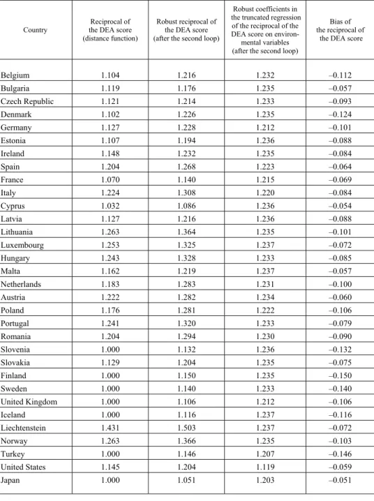
In the presence of an environmental variable, Tables 5 (for an input-oriented model) and 6 (for an output-oriented model) illustrate the re-ranking of countries according to their bias-corrected distance function scores, based on Simar and Wilson’s [2007]
second algorithm for bias-correction of technical efficiency scores in input- and out- put-oriented DEA models (in Simm–Besstremyannaya [2016] implementation).
It should be noted that computations are made in terms of a distance function, that is, the reciprocal of the efficiency score.
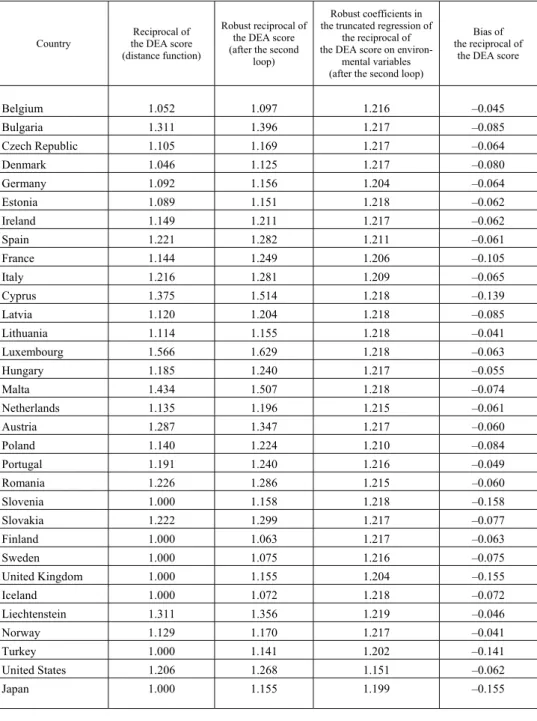
The largest positional changes in Table 5, that is, the most substantial absolute estimated bias of the reciprocal of DEA score, occur for Finland, Turkey, Sweden, and Slovenia, whereas the smallest changes correspond to Japan, the United States, Cyprus, Bulgaria, and Malta. Regarding the output-oriented approach in Table 6, the largest corrections appear in the cases of Slovenia, Japan, the United Kingdom, and Turkey, while the smallest match the cases of Lithuania, Norway, Belgium, and Liechtenstein.
Table 5 Variable returns to scale in DEA with environmental (exogenous) variables – Input efficiency model
Country Reciprocal of the DEA score (distance function)
Robust reciprocal of the DEA score (after the second loop)
Robust coefficients in the truncated regression
of the reciprocal of the DEA score on environ- mental variables (after the second loop)
Bias of the reciprocal of
the DEA score
Belgium 1.104 1.216 1.232 –0.112 Bulgaria 1.119 1.176 1.235 –0.057 Czech Republic 1.121 1.214 1.233 –0.093 Denmark 1.102 1.226 1.235 –0.124 Germany 1.127 1.228 1.212 –0.101 Estonia 1.107 1.194 1.236 –0.088 Ireland 1.148 1.232 1.235 –0.084 Spain 1.204 1.268 1.223 –0.064 France 1.070 1.140 1.215 –0.069 Italy 1.224 1.308 1.220 –0.084 Cyprus 1.032 1.086 1.236 –0.054 Latvia 1.127 1.216 1.236 –0.088 Lithuania 1.263 1.364 1.235 –0.101 Luxembourg 1.253 1.325 1.237 –0.072 Hungary 1.243 1.328 1.233 –0.085 Malta 1.162 1.219 1.237 –0.057 Netherlands 1.183 1.283 1.231 –0.100 Austria 1.222 1.282 1.234 –0.060 Poland 1.176 1.281 1.222 –0.106 Portugal 1.241 1.320 1.233 –0.079 Romania 1.204 1.294 1.230 –0.090 Slovenia 1.000 1.132 1.236 –0.132 Slovakia 1.129 1.204 1.235 –0.075 Finland 1.000 1.150 1.235 –0.150 Sweden 1.000 1.140 1.233 –0.140 United Kingdom 1.000 1.106 1.212 –0.106
Iceland 1.000 1.116 1.237 –0.116 Liechtenstein 1.431 1.503 1.237 –0.072 Norway 1.263 1.366 1.235 –0.103 Turkey 1.000 1.146 1.207 –0.146 United States 1.145 1.204 1.119 –0.059
Japan 1.000 1.051 1.203 –0.051
Table 6 Variable returns to scale in DEA with environmental (exogenous) variables – Output efficiency model
Country Reciprocal of the DEA score (distance function)
Robust reciprocal of the DEA score (after the second
loop)
Robust coefficients in the truncated regression of
the reciprocal of the DEA score on environ-
mental variables (after the second loop)
Bias of the reciprocal of
the DEA score
Belgium 1.052 1.097 1.216 –0.045 Bulgaria 1.311 1.396 1.217 –0.085 Czech Republic 1.105 1.169 1.217 –0.064 Denmark 1.046 1.125 1.217 –0.080 Germany 1.092 1.156 1.204 –0.064 Estonia 1.089 1.151 1.218 –0.062 Ireland 1.149 1.211 1.217 –0.062 Spain 1.221 1.282 1.211 –0.061 France 1.144 1.249 1.206 –0.105 Italy 1.216 1.281 1.209 –0.065 Cyprus 1.375 1.514 1.218 –0.139 Latvia 1.120 1.204 1.218 –0.085 Lithuania 1.114 1.155 1.218 –0.041 Luxembourg 1.566 1.629 1.218 –0.063 Hungary 1.185 1.240 1.217 –0.055 Malta 1.434 1.507 1.218 –0.074 Netherlands 1.135 1.196 1.215 –0.061 Austria 1.287 1.347 1.217 –0.060 Poland 1.140 1.224 1.210 –0.084 Portugal 1.191 1.240 1.216 –0.049 Romania 1.226 1.286 1.215 –0.060 Slovenia 1.000 1.158 1.218 –0.158 Slovakia 1.222 1.299 1.217 –0.077 Finland 1.000 1.063 1.217 –0.063 Sweden 1.000 1.075 1.216 –0.075 United Kingdom 1.000 1.155 1.204 –0.155
Iceland 1.000 1.072 1.218 –0.072 Liechtenstein 1.311 1.356 1.219 –0.046 Norway 1.129 1.170 1.217 –0.041 Turkey 1.000 1.141 1.202 –0.141 United States 1.206 1.268 1.151 –0.062
Japan 1.000 1.155 1.199 –0.155
It can be noticed that in both approaches, there are no exact unity values of bias- corrected distance function scores. For the input-oriented approach, the lowest distance function values are reached by Slovenia, Finland, Sweden, the United Kingdom, Iceland, Turkey, and Japan. The highest distance function values occur for Liechtenstein, Norway, Lithuania, Hungary, and Luxembourg. For the output-oriented approach, the picture is somehow different, with Slovenia, Finland, Sweden, the United Kingdom, Iceland, Turkey, and Japan at one end of the spectrum and Luxembourg, Cyprus, Malta, Bulgaria, and Liechtenstein on the opposite end.
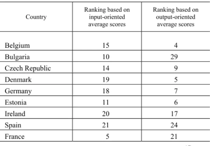
Overall, the robust analysis shows the potential of data biases to distort the pic- ture provided by a standard DEA. Furthermore, to provide a more comprehensive view of the analysis results, Table 7 reports the average ranks based on the bias- corrected methods without and with the environmental variable. Several aspects can be highlighted here. First, there is no single country that displays high levels of effi- ciency in both input- and output-oriented assessments. Some countries, such as Japan, Cyprus, or France, which show good performances in terms of inputs, get worse results when output-based efficiency is considered. For other countries (Lithuania, Belgium, or Norway, etc.), there seems to be a net improvement in effi- ciency with a shift from input-oriented to output-oriented valuation. However, for Latvia, Spain and Italy, the outcomes are, at a higher degree, robust to changes in the perspective of efficiency estimation.
Second, regardless of how efficiency is considered, there are cases (Liechtenstein, Portugal, Romania, Austria, and Luxembourg) that display relative inefficiency in the data sample.
Table 7 Average ranks from the analysis based on bias-corrected
methods without and with an environmental variable Country Ranking based on
input-oriented average scores
Ranking based on output-oriented
average scores
Belgium 15 4 Bulgaria 10 29 Czech Republic 14 9 Denmark 19 5 Germany 18 7 Estonia 11 6 Ireland 20 17
Spain 21 24
France 5 21
(Continued on the next page)
(Continued) Country Ranking based on
input-oriented average scores
Ranking based on output-oriented
average scores
Italy 26 23
Cyprus 2 31
Latvia 16 16
Lithuania 30 8
Luxembourg 28 32
Hungary 29 19
Malta 17 30
Netherlands 22 15
Austria 23 27
Poland 24 18
Portugal 27 20
Romania 25 25
Slovenia 6 14
Slovakia 12 26
Finland 9 1
Sweden 7 3
United Kingdom 3 11
Iceland 4 2
Liechtenstein 32 28
Norway 31 10
Turkey 8 12
United States 13 22
Japan 1 13
4. Final remarks and conclusions
Interpreting the education process as a generator of human capital can raise several objections. One possible objection is that each person is unique, and a child cannot be ‘substituted’ with another. Thus, irrespective of how many pupils are trained, there is no ‘mass production’ in education, but rather a ‘production’ of unique individuals, each possessing their own personal capital. Another conceivable objection is that this type of capital cannot be deconstructed into constituent skills, aptitudes, or knowledge, since it embodies the synergistic outcome of all skills or