O R I G I N A L P A P E R Open Access
Estimating commuting modal split by using the Best-Worst Method
Szabolcs Duleba, Sarbast Moslem and Domokos Esztergár-Kiss*
Abstract
Method:This paper endeavors to introduce a new approach to modal split estimation. In the frame of the research, a customized model of the recently created Best-Worst Method (BWM) is applied to evaluate mode choice alternatives by transport experts. The integrated BWM model is tested on a real-world case study in Budapest, the capital of Hungary, where a small number of selected experts estimate the modal split of three different groups clustered based on the distance of their commuting.
Results:The results clearly demonstrate the popularity of public transport among all groups, while car is estimated to be used primarily by short- and mid-distance commuters. The coherence of the responses is tested along with sensitivity analysis and rank correlation comparison. Moreover, the final results are compared to the official modal split data of the city.
Recommendations:Based on the findings, it can be concluded that the application of BWM results in competitive accuracy compared to the mainstream methodologies, moreover BWM needs significantly less cost and time effort during the survey procedure.
Keywords:Modal split, Multi-criteria decision-making, Best-worst method, Rank correlation
1 Introduction
While operating, and developing urban transport sys- tems, transport planners pay increased attention to the behavior of commuters. Travels going from home to their workplace give a major part of the total urban travel. Commuting mode choice plays a significant role and makes a long-term impact on traffic, emissions, and delays [36]. As commuting is a dominant part of the total travel distance in urban areas, it is worth analyzing the selection of mobility type and the alternatives [25].
The majority of scientific papers approach commuting modal split indirectly through its attributes. In a general mode choice model, first the features of the selection of transport mode are determined, which is followed by the respective weights of these features in the decision, and finally, based on the gained results, the predicted choice of alternative is presented. Consequently, the
identification of the attributes and their significance in mode choice decisions has been in the focus of re- searchers for decades, and different models and ap- proaches have emerged to understand travelers’
attitudes. Tyrinopoulos and Antoniou [41] find that commuters prefer car for their trips. Among many influ- encers, the variable ‘available parking space’ has the highest weight, which is followed by the negatively con- nected ‘crowd on public vehicles’, while the high fare levels or the lack of transport information surprisingly do not discourage citizens from using public transport.
De Jong and Van de Riet [6] emphasize the importance of household income as a key features in mode choice:
higher income motivates families to use private modes for mobility, especially private car. In a more recent re- search, Ko et al. [18] confirm the high car-dependency of high-income commuters, but highlight spatial hetero- geneity as a significant attribute of commute mode choice along with the previous findings of Meurs and Haaijers [28] and Clifford et al. [5].
© The Author(s). 2021Open AccessThis article is licensed under a Creative Commons Attribution 4.0 International License, which permits use, sharing, adaptation, distribution and reproduction in any medium or format, as long as you give appropriate credit to the original author(s) and the source, provide a link to the Creative Commons licence, and indicate if changes were made. The images or other third party material in this article are included in the article's Creative Commons licence, unless indicated otherwise in a credit line to the material. If material is not included in the article's Creative Commons licence and your intended use is not permitted by statutory regulation or exceeds the permitted use, you will need to obtain permission directly from the copyright holder. To view a copy of this licence, visithttp://creativecommons.org/licenses/by/4.0/.
* Correspondence:esztergar@mail.bme.hu
Department of Transport Technology and Economics, Budapest University of Technology and Economics, Műegyetem rkp 3, Budapest 1111, Hungary
The novelty of the present research is the creation and thorough analysis of a Best-Worst Method (BWM) model for mode choice and modal split estimation, con- sidering the problem as a Multi-Criteria Decision- Making (MCDM), where the possible modes are the al- ternatives. In contrast to other methodologies in decision-making, a direct approach is applied in this study. The procedure and analysis are not split into a feature determination section and an alternative evalu- ation section, which results in a more parsimonious sur- vey with short evaluation time and less effort required of the respondents.
Except for reducing time and cost, within the circle of MCDM models, the direct evaluations have the advan- tage of avoiding the double risk of bias in the evaluations because in the indirect models, both the scoring of attri- butes and the scoring of alternatives can be biased. As an example, in case of an Analytic Hierarchy Process (AHP) model [29], the evaluation of the criteria’s weights can be vague as well as the evaluation of the criteria makes an impact on the alternatives. In the BWM model the respondents only need to estimate the modal split proportion of travel modes; thus, the risk of bias can be reduced to one phase.
In this paper, the objective is to test whether the BWM provides applicable results in an expert survey to determine the modal split for commuting. It has to be mentioned that the proposed direct BWM model is not free from bias, but the risk is reduced by the direct evaluation of the alternatives. This paper differs from previous studies in the following major points:
The respondents of the questionnaire are transport experts who are commuters themselves, thus they can evaluate the alternatives with high efficiency.
The commuting modal split is examined as the evaluation of alternative comparisons, thus it can be considered as a synthesis of expert opinions.
In comparison with existing models, the approach of this study requires far less efforts to result in an accurate estimation of the modal split.
The paper is organized as follows. After the introduc- tion, Section 2 presents a review of several scientific pa- pers on commuting mode choice and on the major models applied for analyzing and predicting these types of decisions. In Section 3, the fundamentals of the ap- plied BWM methodology are introduced to justify its se- lection from the wide range of MCDM techniques.
Section 4 introduces the case study of an expert survey for which the created model is applied. Moreover, a comparison of the gained results with the outcomes of a large-scale mobility survey conducted in the same city is provided. While in Section 5, conclusions are drawn,
and suggestions are made for the general usage of BWM in modal split estimation.
2 Review on commuting mode choice
Kotoula et al. [19] try to understand the mode choice decision process and reveal the most appropriate inter- ventions for achieving sustainable transport goals. The scholars’ results verify that distance and time are the most important factors, and the most used transport mode is car and public transport. The same result is provided by Lakatos and Mándoki [20]. They evaluate the long-distance parameters of different transportation modes. The research of Lovejoy and Handy [23] clearly demonstrates that campuses are major trip attractors and have a large commuter population. Regarding a spe- cific group of university student commuters, Rodríguez and Joo [35] find that in the case of North Carolina Uni- versity, car (49.6%) is mostly prioritized, which is followed by bus (17.8%), walking (17.2%), and bicycle (11.6%). Likewise, Zhou [46] reaches to the conclusion that the students at the University of California use mostly car (41.2%), the public transport mode gains 30.9%, while bicycle and walking obtain 24.8%. There are other remarkable studies on university students’ mode choice (e.g., [10, 16,44]) demonstrating the significance and uniqueness of this commuting type. Furthermore, the commuting of other groups is also worth studying.
Shannon et al. [37] investigate the mode choice of uni- versity staff at the University of Western Australia. The researchers conclude that in Zone 1 (less than 1 km), staff members tend to use private cars more and less walking and bicycle than students; in Zone 2 (1–8 km), public transport is less used by the employees than the youth; similarly, in Zone 3 (more than 8 km), public transport is underrepresented, while private car is over- represented by the staff. Most of these models involve a large number of evaluators, and usually, the survey process takes for a rather long time even several months.
The aim of this paper is similar to the listed papers, i.e., to determine the modal split of commuting depending on the distance and to introduce a new methodological approach for investigating the modal share estimation problem.
Basically, there are two large groups of methodological techniques applied to investigate mode choice in the sci- entific literature. Discrete Choice Modelling (DCM) is a general approach which aims to analyze the behavior of a decision-maker [40] when facing the problem of choosing from various travel alternatives with the as- sumption that all individuals strive to maximize their utility [21]. Specifically for commuting mode choice, the fundamental aspect of the model is that decision-makers consider travel time and travel cost minimization as the key features of the choice [30].
A serious limitation of DCM models is that for an ap- propriate analysis, they require a large amount of data.
Generally, more than 1000 observations are necessary for a trustworthy outcome of the models in case of not only the simulated data [14] but the conducted surveys, too [3,39]. De Vos et al. [7] claim that it is an evolution in transportation science to move from the purely utility based models to the integration of more subjective attri- butes (e.g., habits and attitudes). Furthermore, Van Acker et al. [42] agree that lifestyle and personal aspects seem to predict travel mode choice better than those discrete choice models that apply merely objective variables.
Within the circle of DCM techniques, the Stated Pref- erence (SP) type of surveys emerges to integrate trav- elers’ attitude into the modeling [26] and is applied for mode choice, as well [45]. Although DCM with SP pro- vides a more advanced methodology, it cannot deal with the inconsistency of the participants’responses. This in- consistency means a serious bias in preference surveys and is to be reduced by appropriate techniques [13].
The other group of methodologies applied for modal split estimation is the MCDM based models. The con- cept of the MCDM approach is that choosing a certain transport mode is a decision, which has different criteria (e.g., time, cost, comfort) and alternatives (i.e., private car, public transport, bicycle, walking) [11]. The decision-maker considers these criteria with assigning different weights and evaluates the alternatives by con- cerning the attributes; the decision is made based on the scores of the alternatives [15,24]. These models are cap- able of handling the inconsistency of responses; however, these are rather time- and effort-consuming [2]. Consid- ering all boundaries, in the past few years, the MCDM models gained popularity in transport problem evalua- tions and analysis [24,27,31].
A common characteristic of DCM and MCDM models is that in both cases, questionnaire-based surveys, in which participants respond to directed questions, are ap- plied. The limited information on the available transport modes (for DCM) and the lack of motivation and en- thusiasm in responding (for MCDM) can be consid- ered as a serious bias. Consequently, in current research, experts participate in the survey process.
The created model is primarily based on the recently emerged BWM approach [32, 33]. In comparison with other MCDM techniques, BWM is proven to require less pairwise comparisons (especially in contrast to Analytic Hierarchy Process and Analytic Network Process) and to lead to more consistent answers when ranking alternatives. Because of the merits of the ap- proach, BWM is applied in different study areas, e.g., in the creation of tourism development strategy [1], in investment evaluation [4], in making logistics
performance index [34], or in the ranking of airports [38]. However, BWM has not been applied for mode choice analysis so far; thus, the selection of the alter- natives and evaluators, moreover the consistency check of the gained results are cautiously conducted following the latest results of BWM [22].
3 Research method
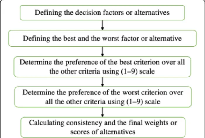
The developed method, like many other MCDM tech- niques, consists of the pairwise comparisons of decision elements. The main difference is that not all compari- sons are completed, only the pairs with the selected best and worst criteria or alternatives are evaluated. The first step is the definition of the existing criteria or alterna- tives in the decision problem. It is followed by the iden- tification of the best and worst criteria or alternatives by the evaluators. Afterward, the pairwise comparisons are applied between the best criterion and other criteria, then between the worst criterion and other criteria. Fi- nally, the weights of all criteria are calculated provided the consistency ratio is acceptable for the pairwise comparisons.
As Fig.1shows, the model works with fixed criteria or al- ternatives determined by the experts at the beginning of the process. Since the second step is to define the best and worst alternatives, the third and fourth evaluation steps are somewhat consistent, but the consistency ratio is higher than other MCDM approaches, especially compared to Analytic Hierarchy Process. However, the fixed position of the best and worst alternatives does not provide the perfect consistency of the evaluations, so a consistency measure is highly recommended in the fifth step.
The general model is customized to the problem of the modal split estimation of commuting, where the word“preference”, which is from the original description of BWM, does not describe the choice of the respond- ent, it rather expresses a professional expert estimation
Fig. 1The main steps of the BWM method to derive the weights of the criteria or alternatives
representing the attitude of a certain group. In the present research, no criteria are applied, only the alter- natives (i.e., the transport modes themselves) are evalu- ated since the study relies on experts’considerations and does not strive to influence their judgements by criteria selection. To provide an overview, the following steps are defined:
– Step 1: Defining the criteria (i.e., decision factors) or alternatives.
– Step 2: Defining the best and worst criteria or alternatives.
– Step 3: Determining the preference of the best criterion over all the other criteria
In this step, the pairwise comparisons between the best criterion or alternative and other criteria or alterna- tives are evaluated by using (1–9) scale, where 1 stands for “equal importance”, and 9 means “extremely more important”. The result of this step is represented by the following vector:AB= (aB1,aB2,…,aBn), whereaBjis the preference of criterionB(i.e., the most important or the best) over criterion j,where aBB= 1, and j= (1, 2, …, n) denotes the number of the criteria (alternatives) in total n.
– Step 4: Determining the preference of the worst criterion over all other criteria
In this step, the pairwise comparisons between the worst criterion or alternative and other criteria or al- ternatives are evaluated by using (1–9) scale, where 1 stands for “equal importance”, and 9 means “ex- tremely more important”. The result of this step is represented by the following vector: AW= (a1W,a2W,
…,anW), where ajW is the preference of criterion W (i.e., the less important or the worst) over the criter- ion j, where aWW= 1, and j= (1, 2, …,n) denotes the number of the criteria in total n.
– Step 5: Calculating consistency and the final weights of criteria or the scores of alternatives
In this step, the final optimal weights (w1;w2;…;wn) of the attributes or alternatives are calculated by com- puting the following model (note that the original BWM is a non-linear model, but here, the linear BWM is pre- sented and applied based on Rezaei [33]):
min maxjwB−aBjwj;wj−ajWwW
ð1Þ s.t.
X
j
wj¼1
wj≥0;for all j
After that, the solution can be obtained by solving the linear programming (LP) formula.
minξl s.t.
wB−aBjwj
≤ξl;for allj wj−ajwww
≤ξl;for allj Xn
jwj¼1;wj≥0;for allj
ð2Þ
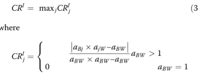
For the consistency measure, the most advanced form, which provides direct feedback for the entries of the evaluations, is the input-based consistency (CRI), which is defined as the following [32]:
CRI ¼ maxjCRIj ð3Þ
where
CRIj¼ aBjajW−aBW
aBWaBW−aBWaBW >1
0 aBW ¼1
8<
:
CRIis the global input-based consistency ratio for all alternatives, while CRIj represents the local consistency level associated with alternativeCRj.
CRI is acceptable in BWM methodology, in case its value is lower than the threshold of the respective input- based consistency determined by the number of the al- ternatives and the extent of the evaluation scale. The consistency thresholds can be obtained for combina- tions, which range from 3 to 9 alternatives with max- imum evaluation grades from 3 to 9 based on the input- based consistency measurement (Table1) [22].
Table 1The threshold for different combinations of scaling and the number of alternatives employing the input-based
consistency measurement Scale Alternative
3 4 5 6 7 8 9
3 0.1667 0.1667 0.1667 0.1667 0.1667 0.1667 0.1667 4 0.1121 0.1529 0.1898 0.2206 0.2577 0.2577 0.2683 5 0.1354 0.1994 0.2306 0.2546 0.2716 0.2844 0.2960 6 0.1330 0.1990 0.2643 0.3044 0.3144 0.3221 0.3262 7 0.1294 0.2457 0.2819 0.3029 0.3144 0.3251 0.3403 8 0.1309 0.2521 0.3154 0.3108 0.3408 0.3620 0.3657 9 0.1359 0.2681 0.3337 0.3517 0.3517 0.3620 0.3662
This ratio can be calculated for individual evaluators, prior to the aggregation of the scores within a certain evaluator group by computing the geometric mean of the individual ratings.
To analyze the inner consistency of the responses of dif- ferent groups, the Kendall rank correlation method [17] is selected. This method estimates the similarity degree for different rankings by taking the average squared difference of the alternatives’ positions. Kendall’s coefficient of con- cordance (K) has a range between 0 and 1, and it can be adopted by applying the following equation:
K¼ 12S
m2ðn3−nÞ ð4Þ
whereS is a sum-of-squares statistic deviations over the row sums of rankingAi, and it can be obtained from the following equations:
S¼Xn
i¼1ðAi−AÞ2 ð5Þ
Ai¼Xm
j¼1rij ð6Þ
where A is the mean of the Ai values, Ai is the aggre- gated ranking of the alternativei, rijis the rank given to alternativeiby the evaluator groupj,mis the number of rater groups ratingnalternatives.
R¼m nð þ1Þ
2 ð7Þ
4 Results
4.1 The framework of the case study
The created BWM model is tested in a case study aim- ing to estimate commuter modal split. MOVECIT pro- ject aims to support sustainable decisions of employees concerning commuting to workplace. This paper pre- sents one of the evaluation steps of the project, more specifically, the evaluation of expert questionnaires. In- formation to estimate commuting is gathered by a ques- tionnaire, which was distributed between 2016 and 2019 among transportation experts, who are employees of an examined university in Budapest as well as teach and conduct research on urban mobility. Thus, 56 faculty members are invited to participate in the evaluation process. The transport experts have to evaluate modal split, travel behavior, and various aspects of mode choice. The participants are clustered into three groups based on their commuting distance assuming that the experts can estimate the modal split for their own com- muting group. There are 26 short-, 21 mid-, and 9 long- distance commuters in the sample.
Usually, in a mode choice model, several mobility types are compared. In the work of De Luca and Di Pace [8], car, car-pooling, and bus are considered, while De Vos et al. [9]
examine car, public transport, walking, and bicycle. Wang and Hu [43] focus on such modes as car, public transport, and teleworking. As a combination of the above mentioned options, in the survey of this research, six mobility types are considered (i.e., Public Transport, Car, Car-Pooling, Walk- ing, Bicycle, and Home Office). Based on the selected com- muting alternatives and according to the BWM logic, the following questionnaire is applied:
“From how far do you commute to work?”
“Select the highest and lowest estimated modal shares of mobility types for commuting!”
“Evaluate the other types with respect to the highest modal share by using (1-9) scale!”
“Evaluate the other types with respect to the lowest modal share type by using (1-9) scale!”
4.2 An example of evaluation with BWM method
Examples of evaluators’estimations regarding the modal shares of mobility types are presented.
Table 2 demonstrates an example scoring of a re- spondent related to the highest estimated modal share of a mobility type, which in this case is public transport.
The lower number indicates the closeness of the alterna- tive to the best one (i.e., the highest estimated modal share in this case). The evaluator indicates home office as a slightly less attractive choice than public transport and car-pooling as the least attractive option to com- mute to work. The higher score represents the larger gap between the alternative mode and the highest esti- mated modal share mode.
Table3demonstrates a respondent’s scoring related to the lowest estimated modal share of a mobility type, which in this case, is car-pooling. It receives the lowest rank, and due to the BWM procedure, all alternatives have to be compared to the least preferred option (i.e., the lowest estimated modal share in this case). The high score of public transport shows that the largest gap is between this mode and the lowest estimated mode. The evaluator expresses a relatively high estimation to car usage, while bicycle gains slightly more points than the lowest estimated mobility type.
The detailed calculation of mobility type alternative’s scores for this example is demonstrated asw= {w1,w2,w3, w4,w5,w6} computed by applying the BWM LP (see Eq.1):
minξ
w1−1w1≤ξ;w1−3w2≤ξ;w1−9w3≤ξ;w1−4w4≤ξ; w1−6w5≤ξ;w1−2w6≤ξ;w3−7w2≤ξ;w3−5w4≤ξ; w3−3w5≤ξ;w3−5w6≤ξw1þw2þw3þw4þw5
þw6¼1w1≥0;w2≥0;w3≥0;w4≥0;w5≥0;w6≥0: The weight scores for this specific evaluation are the following normalized values:
w¼f0:3844;0:1551;0:0337;0:1163;0:0775;0:2327g:
4.3 The evaluation of the case study with the BWM method
In the real-world case study, 56 experts are involved as the total sample. This sample is divided into three groups based on the commuting distance from home to the campus.
short-distance commuters from 1 to 10 km with 26 evaluators,
mid-distance commuters from 10 to 40 km with 21 evaluators,
long-distance commuters from over 40 km with 9 evaluators.
Being experts, the respondents do not indicate their personal experience based estimation, but they are asked to represent a general commuter attitude, thus estimating the mode share from a distance. As a re- sult, based on their professional experience and their own daily travel practice, the experts have to make the scoring during the survey and ultimately provide a modal split estimation. This is calculated based on the responses by using a 1 to 10 scale and an arith- metic mean for both the highest and the lowest modal share cases. After computing the scores of the mobility alternatives for each evaluator and calculat- ing the consistency, the scores for each group are ag- gregated by utilizing the geometric mean. Based on the aggregated answers for all three groups separately and for the total sample, the following results can be presented:
The mobility type with the highest modal share is public transport followed by car.
The mobility type with the lowest modal share is car-pooling followed by bicycle.
The consistency ratio is acceptable for all responses with a value between 0 and 1 in all cases.
4.4 The result of commuters with short travel distance In this group, there are 26 evaluators who are short- distance commuters (i.e., Group 1). After the aggrega- tion of the responses, the results are the followings:
The mobility type with the highest modal share is public transport followed by car.
The mobility type with the lowest modal share is car-pooling followed by bicycle.
Figure 2 demonstrates the normalized scoring BWM result of each transport mode gained by the pairwise comparisons of the respondents from short-distance commuters (i.e., Group 1).
In case of short distance commuting, the highest modal share estimation is for public transport probably due to its relative cheapness and availability. Interestingly, bicycle be- comes underrepresented in the estimation, but it offers great potential for promoting this transport mode for short- distance commuters. Walking is relatively highly estimated, which might be due to its beneficial health and emission ef- fect. Car-pooling is not highly estimated by this respondent sample and do not gain much attention from the evaluators.
4.5 The result of commuters with mid travel distance In this group, 21 evaluators, who are mid-distance com- muters (i.e., Group 2), are involved. After the aggrega- tion of the responses, the results are the followings:
The mobility type with the largest modal share is public transport followed by car.
The mobility type with the smallest modal share is car-pooling.
Figure 3 demonstrates the normalized scoring BWM result of each transport mode gained by the pairwise comparisons of the respondents from mid-distance com- muters (i.e., Group 2).
In this group, public transport is the most estimated choice, which can be well justified based on its low cost and relatively low travel time on average. Bicycle receives a higher estimation than in case of short-distance commuters. Car- pooling is very low estimated by the respondents commuting Table 2Example of evaluating all mobility types compared to the highest share mobility type
Mobility type Public Transport (w1)
Car (w2)
Car-Pooling (w3)
Walking (w4)
Bicycle (w5)
Home Office (w6)
Evaluation 1 3 9 4 6 2
Table 3Example of evaluating all mobility types compared to the lowest share mobility type Mobility type Public Transport
(w1)
Car (w2)
Car-Pooling (w3)
Walking (w4)
Bicycle (w5) Home Office (w6)
Evaluation 9 7 1 5 3 5
from longer distance. All in all, a slight difference can be de- tected compared to the results of Group 1.
4.6 The result of commuters with long travel distance This group includes 9 evaluators, who are long-distance commuters (i.e., Group 3). After the aggregation of the responses, the results are the followings:
The mobility type with the highest modal share is public transport.
The mobility type with the lowest modal share is car-pooling followed by bicycle.
Figure 4 demonstrates the normalized scoring BWM result of each transport mode gained by the pairwise comparisons of the respondents from long-distance commuters (i.e., Group 3).
The results are similar to the previous cases except for the role of home office. It is visible that in case of longer distance, the evaluators consider the home office solu- tion much better. Interestingly, public transport remains the most significant estimation even if the distance is raised. The results clearly show the awareness of the evaluators regarding the environment and sustainability.
4.7 Final scores and ranks for all groups
By applying the BMW method, not only the estimated ranking of transport mode alternatives can be obtained, but a quantified list of experts’ estimation for mobility types, as well. Table4presents the weights for the com- muting alternatives per group and for the whole sample.
Note that for commuting from larger distances, the mode of walking is not offered due to its unrealistic situ- ation. Consequently, for Group 2 and Group 3, five al- ternatives are provided.
Figure 5 shows the graphical comparison of the scor- ing results of the estimated modal split for the three commuting groups. These are the numbers derived from the BWM pairwise comparisons; consequently, the higher column demonstrates the higher modal split ex- pectation toward the mobility type. It is visible that the scores are correlated, and it might be worth to examine the degree of similarity in mode choice ranking among short-, mid-, and long-distance commuters.
For this purpose, the Kendall rank correlation method, which calculates a similarity score for different rankings by taking the average squared difference of the alterna- tives’positions based on the number of evaluator groups and the number of the decision alternatives, is selected.
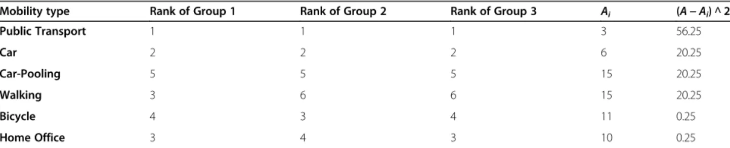
Note that for Group 2 and Group 3, the walking mode is positioned to the 6th place to be capable of conduct- ing the concordance analysis.
In Table5, the final ranking of the mobility types with the number of alternatives (n= 6) and the number of groups (m = 3) are presented. By applying Eq. 4, the Kendall concordance degree (K = 0.746) is obtained, which indicates a strong agreement among the different evaluator groups. This remark can be made since the value of 1 would mean 100% similarity, and all values above 0.5 can be considered as high concordance; thus, 0.746 represents a good result.
Fig. 2The normalized scoring BWM result of the mobility types for Group 1
Fig. 3The normalized scoring BWM result of the mobility types for Group 2
Fig. 4The normalized scoring BWM result of the mobility types for Group 3
Table 4The normalized scoring BWM results of the mobility types
Mobility type Group 1 Group 2 Group 3 All groups Public Transport 0.4860 0.4600 0.5141 0.4863
Car 0.1990 0.2918 0.2074 0.2291
Car-Pooling 0.0418 0.0481 0.0451 0.0449
Walking 0.0993 – – 0.0993
Bicycle 0.0745 0.1167 0.0778 0.0878
Home Office 0.0993 0.0833 0.1556 0.1088
Table 5 clearly demonstrates the dominance of public transport in commuting for all groups. Car-pooling is the least scored option for the largest travel distance, where it could be especially well utilized. While car is mostly expected for all commuters regardless the dis- tance. Working from home gets middle-level scores from all groups of experts. Bicycle might be a popular mode among commuters traveling 10 to 40 km, but there is room for improvement, and primarily short- distance commuters can be motivated to use bicycle more often.
Based on the results, some suggestions how to motiv- ate commuters to utilize more sustainable transport modes can be concluded for transport planners. Al- though the correlation among the three types of com- muting is rather strong, some distinctions can be made in a campaign for sustainable commuting. The innova- tive idea of car-pooling can possibly be popular among short- and mid-distance commuters. University com- muters tend to use bike from middle distance. Thus, a focused campaign on bicycle usage might be effective for this group of employees.
In case the public transport is not available, as a second option, walking, bicycle, or home office might be recom- mended for staff commuters in short- and mid-distance.
On the other hand, for long-distance commuters none of the other alternatives might substitute the public transport
service effectively. The higher utilization of public trans- port might be attractive especially for employees living in mid-range distance, so a focused campaign should target them as potential new users of the mode.
4.8 Input-based consistency
The consistency (CRI) for various individuals in all groups is computed by using the model and Eq.3.
The global consistency for each comparison in Group 1 based on the input-based consistency is accepted since each comparison is all below the threshold of 0.3517, which refers to the 6 alternatives and 9 scale combina- tions (Table 1). The global consistency for each com- parison in Group 2 based on the input-based consistency is accepted sinceeach comparison is are all below the threshold of 0.3337, which refers to 5 alterna- tives and 9 scale combinations (Table 1). The global consistency for each comparison in Group 3 based on the input-based consistency is accepted since each com- parison is all below the threshold of 0.3337, which refers to 5 alternatives and 9 scale combinations (Table1).
To illustrate the input-based consistency measure- ment, an example, which is introduced in subsection
“4.2. Example evaluation with BWM method”, is pre- sented (Table6). In this case, the mobility type with the highest estimated modal share is public transport and the lowest estimation belongs to car-pooling. The pair- wise comparison vectors ofABOand AOW are presented in the second and third rows. By using the input-based consistency measurement as in Eq.3, theCRIj values are represented in the fourth row of Table6.
From Table 6, by using Eq. 3, the global CRI = 0.167 can be found, and it is acceptable since the value is below the threshold of 0.3517, which refers to 6 alterna- tives and 9 scale combinations (Table1).
5 Discussion
A comparison with real-world observed data can provide an appropriate validation of the proposed methodology and the survey process. The official data on the modal split of the examined city are presented by EPOMM [12]. The European Platform on Mobility Management
Fig. 5The estimated modal split of the mobility types for all groups in percentage (%)
Table 5The final ranking of mobility types and concordance degree among the evaluators
Mobility type Rank of Group 1 Rank of Group 2 Rank of Group 3 Ai (A−Ai) ^ 2
Public Transport 1 1 1 3 56.25
Car 2 2 2 6 20.25
Car-Pooling 5 5 5 15 20.25
Walking 3 6 6 15 20.25
Bicycle 4 3 4 11 0.25
Home Office 3 4 3 10 0.25
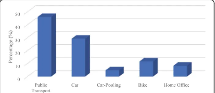
(EPOMM) prepares a modal split in every 10 years. In Budapest, the latest large-scale mobility survey was con- ducted in 2014, and the following proportions of trans- port modes were determined (Fig.6).
Although the data refer to the total modal split rather than specifically to commuting (however, the dominant part of the total travelers in Budapest are commuters), the similarities between the large-scale mobility survey and the cheap and short-time survey of this research are definitely visible. More interestingly, not only the rank- ing (i.e., in case of short-distance commuting, the pos- ition of public transport, car, walking, and bicycle is exactly the same), but the weights, especially in case of the most popular modes (i.e., public transport and car) are also similar. In the model of this study, public trans- port results in the 46–51% of the total modal split, while in the EPOMM survey, it is 45%. Moreover, car receives 20–29% in the results of this research and 35% in the EPOMM survey.
Due to the appearance of very similar modal share re- sults, the risk of coincidence can be considered low in the results of the case study and the large-scale mobility survey. It means that in terms of comparison, both the ranking of the mobility types and the estimated modal shares are very similar for the case study and for the large-scale mobility survey, which justifies the elaborated method.
After gaining the BWM results, a sensitivity analysis is performed for all groups with the aim of checking the robustness of the framework and of eliminating any
possible biases. For Group 1, the score of the public transport alternative is decreased gradually from 0.486 to 0.3. This could be considered as a significant modifi- cation in any MCDM techniques, just as in BWM, in the case of six alternatives. Certainly, the scores of the other alternatives are adjusted to keep the value of 1 for the total sum of the weight scores. Thus, the scores of the other alternatives are changed accordingly.
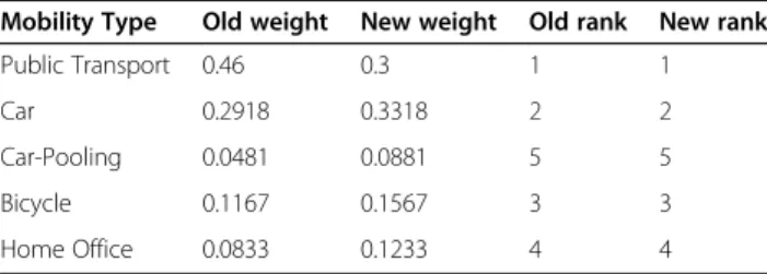
As a result, Table 7 shows stability in the ranking, which indicates the robustness of the framework. Even though the change of the first-ranked mobility type is significant, the ranking of commuting types remains un- changed for all six types. The same steps with the same threshold value of 0.3 for public transport are conducted to check the robustness for Group 2 and Group 3. It could be concluded that the analysis is free from any biases and the results are robust, as presented in Tables 8and9.
The successful application of the BWM technique for a commuting modal split estimation is verified by vari- ous measurable aspects.
First, the calculated input-based consistencies for all comparisons in all three groups are strongly acceptable, which indicates the reliability of the experts’ responses and the validity of the applied BWM model.
Second, the conducted Kendall rank correlation sup- ports the assumption that the difference among the modal estimation of various commuting groups (based on the commuting distance) might not be significant;
thus, a strong correlation among the groups may be expected.
Third, the sensitivity analysis proves that the ranking of all groups is stable, even with a relatively large modifi- cation on the weight of the highest scored mobility type Table 6The evaluations and input-based consistency ratio of each mobility type
Mobility type Public Transport
(w1)
Car (w2)
Car-Pooling (w3)
Walking (w4)
Bicycle (w5)
Home Office (w6)
Mobility type with highest modal share evaluation 1 3 9 4 6 2
Mobility type with lowest modal share evaluation 9 7 1 5 3 5
Input-based consistency 0 0.167 0 0.153 0.125 0.014
Fig. 6The official modal split data from Budapest by EPOMM [12]
Table 7Weight scores and ranking after the sensitivity check for Group 1
Mobility Type Old weight New weight Old rank New rank
Public Transport 0.486 0.3 1 1
Car 0.199 0.2362 2 2
Car-Pooling 0.0418 0.0790 5 5
Walking 0.0993 0.1365 3 3
Bicycle 0.0745 0.1117 4 4
Home Office 0.0993 0.1365 3 3
cannot cause a ranking reversal; consequently, the re- sults are trustworthy.
6 Conclusion
Modal split estimation by applying the BWM method- ology can be considered as a pioneer work in scientific literature. Considering real-world applications, some benefits and limitations are discovered.
As a benefit, the easy-to-use characteristics of the method have to be emphasized based on the experience of the conducted survey. Furthermore, the relatively high consistency of responses is promising and demonstrates the understandability of the BWM based questionnaire and the pairwise comparison logic. The quantified rela- tions could be considered not for the superior alone but for the inferior alternatives as well as an asset of this ap- proach. The strongest argument for the proposed method is the high similarity with a large-scale mobility survey on modal split.
The case study reveals the estimated choice of com- muters in different groups based on the distance of travel and produced robust results in the aspect of sensi- tivity, consistency, and concordance. The sensitivity ana- lysis shows stability for the relatively large modifications of the final scores; measuring consistency proves the co- herence of the responses, and the concordance calcula- tion indicates the strong agreement of the groups. Thus, all tools of MCDM are applied for validating the rele- vance of the BWM in modal split analysis.
As a limitation, the non-flexibility of the alternatives has to be noted. The list of possible alternatives, i.e., the mode choices, could not be extended by the evaluators;
thus, they have to use the provided alternative list.
Consequently, before all BWM survey, a thorough selec- tion of the possible transport modes is necessary consid- ering the mode choice options for different commuting situations.
For the entire validation of the model, the comparison with other existing MCDM techniques is missing. It must be emphasized that for this comparison, another survey is necessary to be conducted because the data gained from BWM procedure are not suitable for pro- cessing other widely applied techniques. However, it is highly recommended to analyze the outcomes by using different models.
Furthermore, it is necessary to compare the effective- ness of the estimation over different periods because considering one time interval the similarities can be inci- dental. Even if we presented solely one example, both the inner logic and the outer test are successful, which is more than promising from the aspect of future BWM applications for modal split estimation.
Acknowledgements
The first author acknowledges the support of the János Bolyai Research Fellowship of the Hungarian Academy of Sciences (No.BO/8/20).
Authors’contributions
Szabolcs Duleba and Sarbast Moslem conceptualized the research and created the suitable methodology. Domokos Esztergár-Kiss conducted the survey. Sarbast Moslem calculated the results. In paper writing all authors participated. The author(s) read and approved the final manuscript.
Funding
The paper was prepared within CE 25 MOVECIT project which is supported by the Interreg CENTRAL EUROPE Programme funded under the European Regional Development Fund.
The research reported in this paper and carried out at the Budapest University of Technology and Economics has been supported by the National Research Development and Innovation Fund (TKP2020 Institution Excellence Subprogram, Grant No. BME-IE-MISC) based on the charter of bol- ster issued by the National Research Development and Innovation Office under the auspices of the Ministry for Innovation and Technology.
Availability of data and materials
The datasets used and/or analyzed during the current study are available from the corresponding author on reasonable request.
Declarations
Competing interests
The authors declare that they have no competing interests.
Received: 3 September 2020 Accepted: 3 May 2021
References
1. Abadi, F., Ghasemian, I., Arab, A., & Alavi, A. (2018). Application of best-worst method in evaluation of medical tourism development strategy.Decision Science Letters,7(1), 77–86.https://doi.org/10.5267/j.dsl.2017.4.002.
2. Abastante, F., Corrente, S., Greco, S., Ishizaka, A., & Lami, I. M. (2019). A new parsimonious AHP methodology: Assigning priorities to many objects by comparing pairwise few reference objects.Expert Systems with Applications, 127, 109–120.https://doi.org/10.1016/j.eswa.2019.02.036.
3. Antonini, G., Bierlaire, M., & Weber, M. (2006). Discrete choice models of pedestrian walking behavior.Transportation Research Part B: Methodological, 40(8), 667–687.https://doi.org/10.1016/j.trb.2005.09.006.
Table 8Weight scores and ranking after the sensitivity check for Group 2
Mobility Type Old weight New weight Old rank New rank
Public Transport 0.46 0.3 1 1
Car 0.2918 0.3318 2 2
Car-Pooling 0.0481 0.0881 5 5
Bicycle 0.1167 0.1567 3 3
Home Office 0.0833 0.1233 4 4
Table 9Weight scores and ranking after the sensitivity check for Group 3
Mobility Type Old weight New weight Old rank New rank
Public Transport 0.5141 0.3 1 1
Car 0.2074 0.2609 2 2
Car-Pooling 0.0451 0.0986 5 5
Bicycle 0.0778 0.1313 4 4
Home Office 0.5141 0.3 1 1
4. Askarifar, K., Motaffef, Z., & Aazaami, S. (2018). An investment development framework in Iran’s seashores using TOPSIS and best-worst multi-criteria decision making methods.Decision Science Letters,7(1), 55–64.https://doi.
org/10.5267/j.dsl.2017.4.004.
5. Clifford, S., Blackledge, D., May, T., Jopson, A., Sessa, C., & Haon, S. (2005).
Final report. Deliverable 11 of the project PLUME (planning and urban mobility in Europe), European Comission 5th framework Programme.
6. De Jong, G., & Van de Riet, O. (2008). The driving factors of passenger transport.European Journal of Transport and Infrastructure Research,8(3), 227–250.https://doi.org/10.18757/ejtir.2008.8.3.3348.
7. De Vos, J., Mokhtarian, P. L., Schwanen, T., & Van Acker, V. (2016). Travel mode choice and travel satisfaction: bridging the gap between decision utility and experience utility.Transportation,43(5), 771–796.https://doi.org/1 0.1007/s11116-015-9619-9.
8. De Luca, S., & Di Pace, R. (2015). Modelling users’behavior in inter-urban car-sharing program: A stated preference approach.Transportation Research Part A: Policy and Practice,71, 59–76.https://doi.org/10.1016/j.tra.2014.11.001.
9. De Vos, J., Derudder, B., Van Acker, V., & Witlox, F. (2012). Reducing car use:
Changing attitudes or relocating? The influence of residential dissonance on travel behavior.Journal of Transport Geography,22, 1–9.https://doi.org/10.1 016/j.jtrangeo.2011.11.005.
10. Delmelle, E. M., & Delmelle, E. C. (2012). Exploring spatio-temporal commuting patterns in a university environment.Transport Policy,21, 1–9.
https://doi.org/10.1016/j.tranpol.2011.12.007.
11. Duleba, S., Mishina, T., & Shimazaki, Y. (2012). A dynamic analysis on public bus transport’s supply quality.Transport,27(3), 268–275.https://doi.org/10.3 846/16484142.2012.719838.
12. EPOMM (2014) Modal split in Budapest, Retrieved from:http://tems.epomm.
eu/result_city.phtml?city=341&map=1, Accessed: 20 Jan 2021.
13. Ghorbanzadeh, O., Moslem, S., Blaschke, T., & Duleba, S. (2019). Sustainable urban transport planning considering different stakeholder groups by an interval-AHP decision support model.Sustainability,11(1), 9.https://doi.org/1 0.3390/su11010009.
14. Guevara, C. A. (2018). Overidentification tests for the exogeneity of instruments in discrete choice models.Transportation Research Part B:
Methodological,114, 241–253.https://doi.org/10.1016/j.trb.2018.05.020.
15. Jadranka, J., & Maja, P. (2001). Modal split modeling using multi-criteria analysis and discrete fuzzy sets.Yugoslav Journal of Operations Research, 11(2), 221–233.
16. Klockner, Z. A., & Friedrichsmeier, T. (2011). A multi-level approach for travel mode choice–How person characteristics and situation specific aspects determine car use in a student sample.Transportation Research Part F: Traffic Psychology and Behaviour,14(4), 261–277.https://doi.org/10.1016/j.trf.2011.
01.006.
17. Kendall, M. G., & Smith, B. B. (1939). The problem of m rankings.Annals of Mathematical Statistics,10(3), 275–287.https://doi.org/10.1214/aoms/11 77732186.
18. Ko, J., Lee, S., & Byun, M. (2019). Exploring factors associated with commute mode choice: An application of city-level general social survey data.
Transport Policy,75, 36–46.https://doi.org/10.1016/j.tranpol.2018.12.007.
19. Kotoula, K., Sialdas, A., Botzoris, G., Chaniotakis, E., Salanova, G., & J. M. (2018).
Exploring the effects of university campus decentralization to students’ mode choice.Periodica Polytechnica Transportation Engineering,46(4), 207– 214.https://doi.org/10.3311/PPtr.11641.
20. Lakatos, A., & Mándoki, P. (2019). Evaluation of traveling parameters in parallel long-distance public transport.Periodica Polytechnica Transportation Engineering,49(1), 74–79.https://doi.org/10.3311/PPtr.14731.
21. Le Pira, M., Marcucci, E., Gatta, V., Ignaccolo, M., Inturri, G., & Pluchino, A.
(2017). Towards a decision-support procedure to foster stakeholder involvement and acceptability of urban freight transport policies.European Transport Research Review,9(4), 54.https://doi.org/10.1007/s12544-017-02 68-2.
22. Liang, F., Brunelli, M., & Rezaei, J. (2019). Consistency issues in the best worst method: Measurements and thresholds.Omega,102175, 102175.https://doi.
org/10.1016/j.omega.2019.102175.
23. Lovejoy, K., & Handy, S. L. (2011).Mixed methods of bike counting for better cycling statistics: The example of bicycle use, abandonment, and theft on the UC Davis campus. Washington DC: 90th annual meeting of the Transportation Research Board.
24. Macharis, C., & Bernardini, A. (2015). Reviewing the use of multi-criteria decision analysis for the evaluation of transport projects: Time for a multi-
actor approach.Transport Policy,37, 177–186.https://doi.org/10.1016/j.tra npol.2014.11.002.
25. Malokin, A., Circella, G., & Mokhtarian, P. L. (2019). How do activities conducted while commuting influence mode choice? Using revealed preference models to inform public transportation advantage and autonomous vehicle scenarios.Transportation Research Part A: Policy and Practice,124, 82–114.https://doi.org/10.1016/j.tra.2018.12.015.
26. Marcucci, E., Stathopoluos, A., Gatta, V., & Valeri, E. (2012). A stated ranking experiment to study policy acceptance: The case of freight operators in Rome’s LTZ.ScienzeRegionali,11(3), 11–30.https://doi.org/10.3280/SCRE2012-003002.
27. Mardani, A., Zavadskas, E. K., Khalifah, Z., Jusoh, A., & Nor, K. M. (2016).
Multiple criteria decision-making techniques in transportation systems: A systematic review of the state of the art literature.Transport,31(6), 359–385.
https://doi.org/10.3846/16484142.2015.1121517.
28. Meurs, H., & Haaijers, R. (2001). Spatial structure and mobility.Transportation Research Part D: Transport and Environment,6(6), 429–446.https://doi.org/1 0.1016/S1361-9209(01)00007-4.
29. Moslem, S., Ghorbanzadeh, O., Blaschke, T., & Duleba, S. (2019). Analysing stakeholder consensus for a sustainable transport development decision by the fuzzy AHP and interval AHP.Sustainability,11(12), 3271.https://doi.org/1 0.3390/su11123271.
30. Owen, A., & Levinson, D. M. (2015). Modeling the commute mode share of transit using continuous accessibility to jobs.Transportation Research Part A:
Policy and Practice,74, 110–122.https://doi.org/10.1016/j.tra.2015.02.002.
31. Pérez, J. C., Carillo, M. H., & Montoya-Torres, J. R. (2015). Multi-criteria approaches for urban passenger transport systems: A literature review.Annals of Operations Research,226(1), 69–87.https://doi.org/10.1007/s10479-014-1681-8.
32. Rezaei, J. (2015). Best-worst multi-criteria decision-making method.Omega, 53, 49–57.https://doi.org/10.1016/j.omega.2014.11.009.
33. Rezaei, J. (2016). Best-worst multi-criteria decision-making method: Some properties and a linear model.Omega,64, 126–130.https://doi.org/10.1016/
j.omega.2015.12.001.
34. Rezaei, J., van Roekel, W. S., & Tavasszy, L. (2018). Measuring the relative importance of the logistics performance index indicators using best worst method.Transport Policy,68, 158–169.https://doi.org/10.1016/j.tranpol.2018.05.007.
35. Rodríguez, J. A., & Joo, J. (2004). The relationship between non-motorized mode choice and the local physical environment.Transportation Research Part D: Transport and Environment,9(2), 151–173.https://doi.org/10.1016/j.
trd.2003.11.001.
36. Schwanen, T., & Mokhtarian, P. L. (2005). What affects commute mode choice: Neighborhood physical structure or preferences toward neighborhoods?Journal of Transport Geography,13(1), 83–99.https://doi.
org/10.1016/j.jtrangeo.2004.11.001.
37. Shannon, T., Giles-Corti, B., Pikora, T., Bulsara, M., Shilton, T., & Bull, F. (2006).
Active commuting in a university setting: Assessing commuting habits and potential for modal choice.Transport Policy,13(3), 240–253.https://doi.org/1 0.1016/j.tranpol.2005.11.002.
38. Shojaei, P., Haeri, S. A. S., & Mohammadi, S. (2018). Airport evaluation and ranking model using Taguchi loss function, best-worst method and VIKOR technique.Journal of Air Transport Management,68, 4–13.https://doi.org/1 0.1016/j.jairtraman.2017.05.006.
39. Tao, X., & Zhu, L. (2020). Meta-analysis of value of time in freight transportation: A comprehensive review based on discrete choice models.
Transportation Research Part A: Policy and Practice,138, 213–233.https://doi.
org/10.1016/j.tra.2020.06.002.
40. Train, K. E. (2009).Discrete choice methods with simulation. United Kingdom, ISBN: 9780511805271: Cambridge University Press.https://doi.org/10.1017/
CBO9780511805271.
41. Tyrinopoulos, Y., & Antoniou, C. (2013). Factors affecting modal choice in urban mobility.European Transport Research Review,5(1), 27–39.https://doi.
org/10.1007/s12544-012-0088-3.
42. Van Acker, V., Van Wee, B., & Witlox, F. (2010). When transport geography meets social psychology: Toward a conceptual model of travel behavior.
Transport Reviews,29(3), 219–240.https://doi.org/10.1080/01441640902943453.
43. Wang, O., & Hu, H. (2017). Rise of interjurisdictional commuters and their mode choice: Evidence from the Chicago metropolitan area.Journal of Urban Planning and Development,143(3), 1–10.https://doi.org/10.1061/
(ASCE)UP.1943-5444.0000381.
44. Whalen, K. E., Páez, A., & Carrasco, J. A. (2013). Mode choice of university students commuting to school and the role of active travel.Journal of Transport Geography,31, 132–142.https://doi.org/10.1016/j.jtrangeo.2013.06.008.
45. Yap, M. D., Correia, G., & Van Arem, B. (2016). Preferences of travelers for using automated vehicles as last mile public transport of multimodal train tips.Transportation Research Part A: Policy and Practice,94, 1–16.https://doi.
org/10.1016/j.tra.2016.09.003.
46. Zhou, J. P. (2012). Sustainable commute in a car-dominant city: Factors affecting alternative mode choices among university students.
Transportation Research Part A: Policy and Practice,46(7), 1013–1029.https://
doi.org/10.1016/j.tra.2012.04.001.
Publisher’s Note
Springer Nature remains neutral with regard to jurisdictional claims in published maps and institutional affiliations.

![Fig. 6 The official modal split data from Budapest by EPOMM [12]](https://thumb-eu.123doks.com/thumbv2/9dokorg/744969.30944/9.892.84.815.150.246/fig-official-modal-split-data-budapest-epomm.webp)