http://siba-ese.unisalento.it/index.php/ejasa/index
e-ISSN: 2070-5948
DOI: 10.1285/i20705948v12n1p153
A measure of adjusted difference between values of a variable
By Dob´o
Published: 26 April 2019
This work is copyrighted by Universit`a del Salento, and is licensed un- der aCreative Commons Attribuzione - Non commerciale - Non opere derivate 3.0 Italia License.
For more information see:
http://creativecommons.org/licenses/by-nc-nd/3.0/it/
DOI: 10.1285/i20705948v12n1p153
A measure of adjusted difference between values of a variable
Andr´ as Dob´ o
∗University of Szeged, Hungary Institute of Informatics
Published: 26 April 2019
Both during academic work and everyday life it is usual to come across such situations, where one has to compute the difference between values of a variable. However, this can be done many ways. For example, the comparison of accuracy values of methods for the solution of a scientific problem is usually done by either looking at how much the absolute difference between the two accuracies in percentage points is, how much their relative difference in percentages is, or how much the relative difference between the two error rates in percentages is. The problem is that these different methods usually give different results, often suggesting contradicting conclusions.
To overcome this problem I propose a novel measure to compute an ad- justed difference (AD) between values of a variable to represent their differ- ence in a better and uniform way, replacing the collection of the previously used conventional measures, and show how the properties of this new measure are superior to those of the other measures.
keywords: Adjusted difference, Integration, Probability density function, Probability distribution, Weight function.
1 Introduction
Either looking at academic work or everyday life, people come across such problems very often, where they have to calculate the difference between two values of a variable.
However, there are many different ways to do this calculation giving different results, often suggesting contradicting conclusions.
∗Corresponding author: dobo@inf.u-szeged.hu
c
Universit`a del Salento ISSN: 2070-5948
http://siba-ese.unisalento.it/index.php/ejasa/index
Let’s take a situation where researchers present their work compared to others’. As- sume a group of researchers develop a methodAfor solving a given problem, which per- forms with 99.9% accuracy on the task. Then later, another group develops a methodB for the same problem, achieving 99.96% accuracy. It is one thing to check whether the difference between the two results is significant at all or not. But even if this difference was significant (say at levelp= 0.05), other researchers might ask the question, whether it was worth the trouble at all to further improve the already almost perfect method?
The answer from the developers of method B would probably be yes, of course, as they would say they have reduced the error of the original method by 60% (relative difference of error in percentages, RDE%=-60; It has to be noted that this measure is only defined in case the domain of the variable in question has an upper bound. Further, in some cases this would actually not be called the relative difference of error in percentages, as an error is actually not defined in that context, rather “error” should be replaced by
“distance from the upper bound of the domain of the variable”. Still, to make it more convenient, I will use the term relative difference of error in percentages [RDE%] in the followings.). On the other hand, the first group of researchers could defend themselves by saying that using the new method increases accuracy by only 0.0601% (relative difference in percentages, RD%=0.0601), which does not really make a difference in practice (and if method B happened to use more resources than method A, then it might even make method B less usable in practice than method A despite its slight superiority in per- formance). And others might have yet another observation, namely that there is a 0.06 percentage point (pp) difference between the two values ([absolute] difference, D=0.06).
Further, probably the most objective (but least informative) observation would be that while the first method had a performance of 99.9%, the second method surpassed this by achieving 99.96%. (But as this statement does not contain any actual comparison of the values, I will not consider this as a measure of difference and will not include this in further discussions.)
In such a situation, what would be the most objective and most informative compar- ison of the performance of the two methods? Moreover, looking at the practical side of the situation, in case method B happened to use more resources than methodA, then methodA orB should be used for the solution of real-life problems in the future?
Further, how would the situation change, if for example the 0.06 pp difference (D) was between the accuracies 60% and 60.06%. In such a case RD% equals 0.1 and RDE%
equals -0.15. Therefore it is obvious, that it is not irrelevant at which point a fixed percentage point D between two values exist. Nor is it irrelevant where a fixed RDE%
takes place: the 60% smaller proportion of faults would yield a very different result, if it was between 60% and 84% of accuracy (a change of 24 pp), than if it is between the previously said 99.9% and 99.96% (a change of 0.06 pp). In case of most problems almost everybody would agree that the difference of 0.06 pp between the accuracies of 99.9% and 99.96% is much more remarkable than that between 60% and 60.06% (even though here the first difference is not really remarkable either, the second one is still much less so), and the RDE% of -60 is much more prominent between the accuracies of 60% and 84% than between the accuracies of 99.9% and 99.96% (here the first difference is rather prominent, while the second one is not really so).
Similar problems in comparison methods can arise in basically any academic or ev- eryday field, for example in case of
• comparing physical or chemical properties of materials,
• looking at the success rates of different medical treatments,
• during the comparison of economic indicators of companies or countries,
• analyzing the changes in crime or accident rates in a country over time,
• comparing the performance of different computer programs for a given task,
• or just trying to choose the most reliable washing machine for your home by com- paring their fault rates,
just to name a few examples.
The lack of and the need for a better difference measure encompassing all important aspects of the difference of values of a variable is easily verified by looking at cutting- edge research, published in even the most influential journals and books in any field, using the above described simple and often misleading measures of either D, RD% or RDE% to compare values of a variable. Very good examples for the usage of such simple measures are Santacruz et al. (2005), Baur et al. (2006), Chapman et al. (2011), Erickson et al. (2011), Harriman et al. (2016) and Rollins et al. (2016) in the field of medical and pharmaceutical sciences, Tasis et al. (2006), Zhu et al. (2007), He et al.
(2012), Huang et al. (2012), Ellsworth et al. (2017) and Rehman et al. (2017) in the field of natural sciences, Mor´e and Wild (2009), Carrasco et al. (2006), Dalal and Triggs (2005), Povey et al. (2011), Burow et al. (2017) and Green and Bremner (2017) in the field of mathematics, engineering and computer science, and Peden et al. (2004), Peresie (2005), H¨am¨al¨ainen et al. (2009), Cremers and Petajisto (2009), Elhauge (2009), Song et al. (2011), Piketty et al. (2017) and Renshon et al. (2018) in the field of economics and social sciences.
So in case of any problem it is one question whether a change or difference in values is significant or not. And it is yet another question whether this (possibly significant) change matters at all and whether it is remarkable or not. In what way can it be determined how remarkable a change is? Well, it can be easily accepted that a change can be considered more significant where the values of the variable are more sparse, hence making a change in the value more difficult. This means that a change should be considered more significant at those places where the values of the variable are less probable, have lower probability of occurring. So this significance can be directly linked to the probability distribution of the variable, having larger significance at those places where the probability density function of the variable has lower values.
And looking back at the previous examples, it is easy to see that this theory is perfectly consistent with the previously phrased intuitions. In case of most problems, the proba- bility density function for the accuracy of the proposed methods would usually have a bell-shaped curve, the probabilities would decrease towards the ends of the bound of the
domain, thus resulting in a more significant change near the bounds. The same situation would also arise in case of variables with semi-bounded or unbounded domain, where the probability would decrease and thus the significance would increase when getting further from the mean of the values.
For example, Piketty et al. (2017) analyze the change of income of different groups of people over time, mostly using the RD% measure for comparison, or simply stating from what value to what value it changed over a period of time, without any real comparison.
However, these methods do not provide a uniform comparison, the findings could be very different if the D measure had been used instead of the RD% measure, and these comparisons do not take the probability distribution of incomes into account. Similar problems arise when comparing road (Peden et al., 2004) and occupational (H¨am¨al¨ainen et al., 2009) accident rates, trying to determine which property of solar cells results in the most increase of energy-conversion efficiency (Green and Bremner, 2017), or which interventions improved breastfeeding practices more (Rollins et al., 2016).
Based on the above observations and conclusions, I have defined a measure that is able to encompass all important aspects of the difference of values of a variable, calculating the difference in a better and uniform way, and therefore which can be employed successfully as a measure of adjusted difference (AD) of values of a variable. To my best knowledge, the measure presented in this article is the first such measure and no similar measures have been proposed yet.
The rest of the paper is structured as follows. In Section 2 I will define the required properties of the measure to be created and constuct a measure satisfying the set prop- erties. Then I will evaluate the created measure with different parameter settings and determine a default setting for the measure in Section 3. After this, I will describe pos- sible ways to extend the constructed measure beyond the comparison of simple values of a continuous variable in Section 4. Finally, I will summarize the article and draw conclusions in Section 5.
2 Implementation of the measure of adjusted difference (AD)
2.1 Defining the required properties for the measure of AD
As it was previously shown, there is a need for a measure of adjusted difference, which can be used to give a uniform way of comparing values of a variable. Before starting to construct this measure, its essential properties and requirements should be determined. I think that in order to get such a difference measure, which has the best possible usability and fits the requirements of the most possible problems, it should satisfy the following basic properties:
1. It should be a function AD:D2 →R, whereD⊆Ris the domain of the variable whose values are to be compared
2. It should return its additive inverse if the order of the two compared values are reversed:
AD(p, q) =−AD(q, p) (1)
3. It should return a positive value if and only if the first value (minuend) is greater than the second (subtrahend):
AD(p, q)>0 ⇔ p > q (2)
4. It should be additive:
AD(p, s) +AD(s, q) =AD(p, q) (3)
Further, these basic properties should be extended with such properties that define the adjustment of the difference returned by the measure. To fulfil all expectations, I think that at least the following properties have to be true:
5. The adjusted difference between an arbitrary pair of points p and q and between another arbitrary pair of points s and t should be equal, if the (unadjusted) differ- ence of the two pairs are the same and the probability density of the variable over the interval [q, p] is pairwise equal to the probability density over the interval [t, s]:
(p−q=s−t ∧ ∀d∈[0, p−q] pdf(q+d) =pdf(t+d))
⇒ AD(p, q) =AD(s, t) (4) wherepdf denotes the probability density function of the variable whose values are compared.
6. The adjusted difference between an arbitrary pair of points p and q should be greater than the adjusted difference between another arbitrary pair of points s and t, if the (unadjusted) difference of the two pairs are the same and the probability density of the variable over the interval [q, p] is pairwise less than the probability density over the interval [t, s]:
(p−q=s−t ∧ ∀d∈[0, p−q] pdf(q+d)< pdf(t+d))
⇒ AD(p, q)> AD(s, t) (5) In my opinion a measure satisfying all the above criteria would have the best possible properties in case of most problems.
2.2 The calculation of AD using a weight function
After having the required properties, the implementation of the AD measure should come. First it should be evaluated how difference is calculated in the normal case, without any adjustment: an absolute difference d always means the same difference, regardless of the location of the two compared values on the domain of the variable.
This means that a change at any point of the domain is the same for all points of the domain, so the change at every point has an equal weight (e.g. 1). Basically it is as if the constant function w(x) = 1 was used as a weight function when calculating the difference.
If there is a weight function, then the weighted difference can be calculated (in case of any weight function) as the definite integral of the weight function between the values to be compared. And if the weight function was equal to the constant functionw(x) = 1, then this integral would simply return the unadjusted difference between the compared values, as expected. Therefore this calculation also applies to the unweighted case, but with a different weight function it can be used to calculate a weighted (adjusted) difference too.
So, the weight function can be applied to calculate the adjusted (weighted) difference by computing its integral between the values to be compared:
AD(p, q) = Z p
q
w(x)dx (6)
wherewis the weight function corresponding to the variable whose values are compared.
This function can be universally used as an adjusted difference measure (with the proper weight function), in case of variables with either bounded, semi-bounded or un- bounded domain. However, when applied to variables with bounded domain, it would also make sense to include some normalization. There are two possible ways for doing this. First, it can be normalized so that the adjusted difference measure calculated for the whole interval of the domain of the variable would be equal to the length of that interval. This would be the adjusted difference with normalization (ADN):
ADN(p, q) = (max−min)Rp
q w(x)dx Rmax
min w(x)dx (7)
,minandmaxdenoting the lower and upper bound of the domain of the variable whose values are compared, respectively.
Further, another possibility is to normalize the measure in a way, such that it returns values ranging from 0 to 1 (both inclusive), thus creating a measure of adjusted difference in percentage points (ADP P):
ADP P(p, q) = Rp
q w(x)dx Rmax
min w(x)dx (8)
2.3 Defining the required properties of an appropriate weight function for the AD measure
So now, in order to fulfil the requirements for theADmeasure, what remains is defining an appropriate weight function. Based on the required properties of the AD measure, let’s figure out what kind of weight function is needed:
1. It should be a function w:D → R, where D ⊆ R is the domain of the variable whose values are to be compared, and w is (Lebesgue) integrable on its whole domain.
2. It should be non-negative:
w(p)≥0 (9)
3. It might only take the value 0 at such a point where the probability density of the variable is equal to infinity:
w(p) = 0 ⇒ pdf(p) =∞ (10)
4. The weight at p should be equal to the weight at q if and only if the probability density of the variable at pand q are equal:
w(p) =w(q) ⇔ pdf(p) =pdf(q) (11)
5. The weight atpshould be greater than the weight atqif and only if the probability density of the variable at pis less than at q:
w(p)> w(q) ⇔ pdf(p)< pdf(q) (12) These properties are both necessary and sufficient to get such an AD measure that satisfies all the required properties set in Section 2.1.
2.4 Choosing an appropriate weight function for the AD measure After defining the required properties for the weight function to be used, let’s construct an appropriate weight function. A very simple solution having the required properties that can easily come to one’s mind would be the multiplicative inverse of the probability density function of the variable:
w(x) = 1
pdf(x) (13)
However, the problem with this function is that it overweighs values with very low prob- ability. Further, in case of variables with a bounded domain, it would result in divergent integrals in case of many widely-used probability density functions. To overcome this, I propose the use of the following extension:
wbn(x) =
logb
1 + 1 pdf(x)
n
(14) By choosing appropriate values for the parametersb(base of the logarithm) andn(expo- nent), this weight function would not overweigh values with low probability. (Although the base of the logarithm [b] can be freely set, it has to be noted that changing it would only result in stretching the function [multiplication with a constant], which would lose
even this effect in case the measure is normalized [ADN and ADP P]. And even in the unnormalized case it would not change the shape of the function other than by a constant multiplication, so changing this parameter does not really have a remarkable effect.) Further, it would only result in divergent integrals in case of some extreme prob- ability density functions, having zero probability over a proper (non-degenerate) interval (e.g. a truncated normal distribution), as then the respective weight function would be infinite over a proper interval, resulting in infinite integrals over finite intervals. In case of such pdfs it is either accepted that the AD measure could be infinite over a finite interval, or, to get a weight function resulting in a convergent integral in case of any possible probability distribution, the weight function can be further extended as follows:
wb;cn (x) =
logb
1 + 1
pdf(x) +c n
(15) wherec is a very small positive constant.
This version of the weight function could never reach an infinite value, thus could never result in a divergent integral. However, I would still not suggest the general use of this measure, as in most cases it would be desirable that the weight function tends to infinity at those places where the probability density is equal to 0, and this is not true in this version.
So in general, I would suggest the weight function defined in Equation 14 to be used, which results in the following parametrizable adjusted difference measures:
ADnb (p, q) = Z p
q
wnb (x)dx (16)
ADNnb (p, q) = (max−min)Rp
q wnb (x)dx Rmax
min wbn(x)dx (17)
ADP Pnb (p, q) = Rp
q wnb (x)dx Rmax
min wbn(x)dx (18)
,minandmaxdenoting the lower and upper bound of the domain of the variable whose values are compared, respectively.
2.5 Proving that the set properties of AD are satisfied
At the beginning of the research a couple of conditions have been set that the AD measure should satisfy, which are detailed in Section 2.1. In this section I will prove that these properties are satisfied by the proposed AD measure. As the satisfaction of all properties can be proved with basic mathematical and logical operations, I will only provide a brief deduction in each case and will not go into too much detail.
Let’s start by proving that the properties for the AD measure set in Section 2.1 are satisfied based on the properties of the weight function set in Section 2.3 and on the properties of integration:
• Property 1 ofAD: satisfied if Property 1 ofw is satisfied
• Property 2 ofAD: satisfied because reversing the limits of integration changes the sign of the definite integral
• Property 3 ofAD: satisfied if Properties 2 and 3 of ware satisfied
• Property 4 ofAD: satisfied because the definite integral is additive
• Property 5 ofAD: satisfied if Property 4 ofw is satisfied
• Property 6 ofAD: satisfied if Property 5 ofw is satisfied
Then, it would be very easy to prove that the chosen weight function truly satisfies the properties set for it in Section 2.3, knowing the properties of the used mathematical operations and that any probability density function has a rangeA⊆R≥0.
So hereby I have proven that the newly proposed AD measure truly satisfies the properties set for it Section 2.1.
3 Evaluation
To test how my measures would work in real-life problems and to be able to choose a general parameter setting that would be suitable in most (non-extreme) situations, a thorough testing with different parameter settings was conducted. In order that the results are easily comparable, it is logical to conduct tests using theADP Pbnmeasure on variables with bounded domain first. A thorough testing with many parameter settings on the most widely-used bounded-domain probability distributions have been done, from which a representative sample of results are summarized in Table 1. As changing the base of the logarithm (b) does not cause any change in the measureADP Pbn(see Section 2.4), the natural logarithm was used in all cases. Further, it has to be noted, that in case of all the probability distributions included in Table 1 their domain is the [0,1] interval, therefore in all these cases theADP Pbnmeasure actually also equals theADNbnmeasure.
When looking at the results in case of the n = 1 parameter setting, then it can be observed that in many cases the difference between the values of the observed variable seems to be overweighed: for example, a difference between 1.0 and 0.99 (an absolute difference of 0.01) results in an ADP P1e(p, q) of around 0.07 in several cases and a difference between 1.0 and 0.9 (an absolute difference of 0.1) results in anADP P1e(p, q) of around 0.3 in case the probability density function had a bell-shape, which seems to be too much in most cases.
On the other hand, setting this parameter to as low asn= 0.25 seems to underweigh the difference in many cases, producing an ADP P0.25e (p, q) less than 0.02 in all cases when considering the difference between 1.0 and 0.99 (an absolute difference of 0.01), and always giving anADP P0.25e (p, q) of less than or equal to 0.15 in case of a difference between 1.0 and 0.9 (an absolute difference of 0.1).
All in all, based on the results of the thorough testing, a parameter setting ofn= 0.5 seems to be about right for most general problems (in case of both bell-shaped and U-shaped probability density functions), so this parameter setting will be used during
further tests. However, this parameter could of course be adjusted in case of problems with special needs.
After choosing the appropriate exponent (n), it should be tested whether the pro- posed adjusted difference measure truly outperforms any previous measure of difference currently in use. Changing the base of the logarithm (b) does not result in anything other than a constant multiplication in case of the unnormalized measure (ADbn) either, therefore changing this parameter does not make much of a difference here either. The natural logarithm seems to be perfectly suitable for the task, so this parameter setting will be used during further tests too.
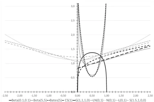
Using the parameter setting detailed above, the different probability density functions and their respective weight functions can be observed in Figures 1 and 2, respectively.
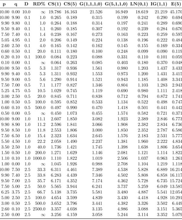
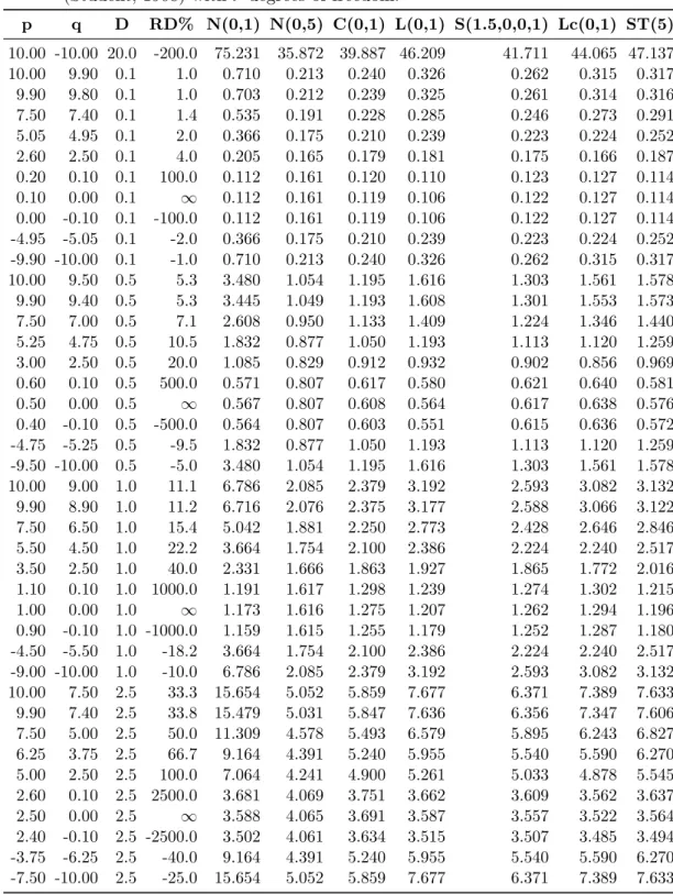
Further, the detailed numerical results of the thorough tests for theAD0.5e (p, q) measure on variables with bounded, semi-bounded as well as unbounded domain can be found in Tables 2, 3 and 4, respectively. In Table 2 both theAD0.5e (p, q) andADP P0.5e (p, q) results are presented, and, because of the [0,1] domain of the probability distributions in- cluded in the table, theADP P0.5e (p, q) results are actually the same as theADN0.5e (p, q) results would be.
In my opinion, this proposed measure is much more suitable for showing the difference between values of a variable than any of the previous measures currently in use. To prove this, let’s test all the measures with the help of a real-world problem. For this, let’s assume that the values presented in Table 2 correspond to the F1-scores of binary classification systems on a given test set with equal number of test cases of both classes.
For our evaluation, let’s consider the following three situations: in the first case there was a binary classification system with an F1-score of 0.25, which was later improved by their creators to achieve an F1-score of 0.3, in the second case an original system with an F1-score of 0.475 was enhanced to having an F1-score of 0.525, while in the third situation the system’s original F1-score of 0.94 was later increased to 0.99.
To be able to evaluate the results, the probability distribution of the performance of the systems needs to be known. Let’s assume that the F1-scores of binary classification systems follow a Beta(5,5) distribution. This means that the probability density function has low values near the bounds of the domain of the variable (near 0 and 1), while having its maximum at the center of the domain (0.5). So there are many mediocre systems, while the better the performance is, the fewer such systems exist.
The better system one wants, the more difficult it is to create, and therefore the least such systems exist. Further, it is equally difficult to create a system with low performance, as in case of binary classification it could easily be transformed into a good system by simply reversing the output labels of the system. On the other hand, the easiest it is to create a system with mediocre performance, for example by creating a system that always returns a randomly chosen class, whose F1-score would converge to 0.5 (because there are equal number of test cases in case of both classes).
Therefore it is pretty safe to assume that the F1-scores of binary classification systems have a symmetric bell-shaped probability distribution (such as the Beta(5,5) distribu- tion). This means that, as it is hard to create a good system, it is even harder to further improve it. Therefore the difference between two large F1-scores should be considered
Figure 1: Probability density functions in case of several probability distributions. Ab- breviations: see Tables 1, 3 and 4.
Figure 2: The respective weight functions in case of several probability distributions.
Abbreviations: see Tables 1, 3 and 4.
very remarkable and the difference between two small F1-scores should be considered equally remarkable. On the other hand, in case of two mediocre F1-scores the difference is much less relevant as it is much easier to improve a system that has a mediocre per- formance. Now let’s see how the original measures of difference and the new measure proposed here follow these properties.
As it can be seen, the measure of absolute difference (D) returns the same value irrespective of where on the domain of the variable the difference is located. It does not consider the possible bounds of the domain of the variable and the probability distribution of the variable (so this measure does not satisfy the previously set Properties 5, 6). So in case of each example pair the absolute difference is the same (0.05), although the relevance of these three differences are not the same at all.
Next, the relative difference in percentages (RD%), irrespective of the possible bounds of the domain of the variable or its probability distribution, puts more weight on those cases where the compared values are closer to 0. Therefore, although the difference between the F1-scores of 0.99 and 0.94 should be more remarkable than the difference between the F1-scores of 0.3 and 0.25 and even so than between those of 0.525 and 0.475, in case of the RD% measure it is the other way around. Further, in case of comparing two small values, it overweighs the difference, and it returns infinity in case the second value is zero irrespective of the first value (except when the two values are equal). In addition, it can also return a negative difference instead of a positive one in case the first value is positive while the other being negative. What is more, this measure does not satisfy the previously set Properties 2, 3 and 4 (of course beside not satisfying Properties 5 and 6 either).
Finally, the relative difference of error in percentages measure (RDE%) puts more weight on those differences that occur near the upper bound of the domain of the variable without taking the probability distribution or the lower bound of the domain of the variable into account. It is correct that the result is the most prominent in case of the (0.99,0.94) pair, however the difference in case of the value pair (0.525,0.475) should not be more prominent than that of the (0.3,0.25) pair. (As opposed to the other measures, here by most prominent actually the smallest [and not the largest] value is meant, as the RDE% measure always returns results with opposing sign compared to the other measures.) Further, this method seems to overweigh the relevance of the difference in case of two values near the upper bound, like in case of the value pair (0.99,0.94).
Moreover, if the first value is actually the upper bound, then the difference is always -100 irrespective of the second value (except when the two values are equal). In addition, this measure can only be used if the domain of the variable has an upper bound. What is more, similarly to the RD% measure, this measure also does not satisfy the previously set Properties 2, 3 and 4 (of course beside not satisfying Properties 5 and 6 either).
As opposed to the other measures, theAD0.5e (p, q),ADN0.5e (p, q) andADP P0.5e (p, q) measures proposed in this article take both the probability distribution of the variable and the possible bounds of the domain of the variable into account. So the comparison between two fixed points would result in different adjusted differences in case of different probability distributions. Further, a fixed absolute difference (D), relative difference in percentages (RD%) or relative difference of error in percentages measure (RDE%) could
also result in different adjusted differences in case of different probability distributions or different locations on the domain of the variable. Finally, the values returned by them for the given three pairs follow the same order as the relevance of the pairs, and they do not overweigh any difference. Therefore these new measures eliminate all the shortcomings of the previous measures, unite their positive properties, and thus constitute much better measures of difference than the previous ones.
Although the measures were only evaluated in detail in case of one problem with a variable with bounded domain and with a given probability distribution, very similar conclusions can be reached in case of problems with a variable with a semi-bounded and unbounded domain, as well as in case of other probability distributions.
To take an example, we can look at the study of Piketty et al. (2017). They give a detailed analysis on how the income of different groups of people have changed over the years in the United States of America. They usually employ the RD% measure for comparison, or they simply state from what value to what value the income of a group of people has changed over a period of time, without any real comparison (in some cases they use ”both” comparison methods, even though the second method cannot really be considered a true comparison method). However, the findings could be very different if the D measure had been used instead of the RD% measure, these measures do not provide a uniform comparison, they do not take the probability distribution of incomes into account, and they do not satisfy the properties set for a decent comparison measure defined in Section 2.1. So by using the newly proposed AD measure one could provide a better, more uniform comparison, satisfying all set set properties for it also taking the probability distribution of incomes into account. Similar conclusions would hold in case of the other examples mentioned in Section 1.
4 Extensions of the AD
bnmeasure to other data types
So far I have shown how the adjusted difference of values of a simple variable with a continuous domain can be calculated. Now let’s see how this simple measure could be extended to be able to be used on other data types too.
4.1 ADnb on discrete variables
Until now, I have implicitly only talked about the difference of values of a continuous variable. And what happens if the variable is discrete rather than continuous? Well, the probability distribution of a discrete variable is defined by a discrete probability mass function instead of a continuous probability density function. To calculate an adjusted difference based on this, I propose two different options.
First, although the domain of a probability mass function is always discrete, the function underlying it can usually be interpreted as a continuous function too. Therefore one logical solution would be to use this continuous version of the probability mass function for the calculations (which can be denoted as cpmf), and this way the same calculations could be used as in case of continuous variables, just the weight function
would change as follows:
wnb (x) =
logb
1 + 1
cpmf(x) n
(19) Second, if it is not possible or desired to interpret the probability mass function as a continuous function, then there is another possibility. In this case the difference between two adjacent discrete values, so basically the interval between them, needs to be weighted, where the value of the weight function is only known at the endpoints of that interval. In the absence of any further information available, the best solution is to use the mean weight of the endpoints of the interval in case of all points of the interval, and do the calculations according to this (actually, this is the same as approximating the integral of an implicitcpmf on the given interval using the trapezoid rule). And if a weighted difference between two adjacent points can be calculated like this, then an adjusted difference between any two points can be calculated by computing the weighted sum of the intervals between the two points. So in this case the calculation of the integral is replaced by the calculation of a weighted sum:
ADnb (p, q) = X
i∈[q,p]
l(i)∗meanwnb (i) (20) , where i runs through all the intervals between the values q and p, l(i) denotes the length of the interval iand:
meanwnb (i) = wnb (lowerend(i)) +wnb (upperend(i))
2 (21)
wbn(x) =
logb
1 + 1
pmf(x) n
(22) , where lowerend(i) and upperend(i) denote the lower and upper endpoints of the in- terval, respectively.
Here the normalized versions of the adjusted difference are calculated as follows:
ADNnb (p, q) = (max−min)P
i∈[q,p]l(i)∗meanwnb (i) P
j∈[min,max]l(j)∗meanwnb (j) (23) ADP Pnb (p, q) =
P
i∈[q,p]l(i)∗meanwnb (i) P
j∈[min,max]l(j)∗meanwnb (j) (24) With this extension of the AD measure, one can, for example, determine which inter- ventions have been the most influential in reducing the number of road accidents, based on the implementation year of the interventions and on the statistics of road accidents for a sequence of years (e.g. from Peden et al., 2004, Ruikar et al., 2013 or Eurostat, 2018), from which the probability mass function of road accidents can be estimated.
Similarly to the continuous case, theADmeasure on discrete variables could result in infiniteADvalues over a finite interval in case of such pmfs that have a zero probability at any point, which would result in an infinite weight at that point. This could be avoided with the same extension to the weight function as in the continuous case.
4.2 ADnb on intervals of a variable
It is also a common situation that one has to compute the difference between intervals, for example between two confidence intervals. Here I also propose two different versions on computing the adjusted difference between intervals of a variable. The first version uses the standard interval arithmetic, namely:
ADnb ([p, q],[s, t]) = [ADnb (p, t), ADnb (q, s)] (25) However, I also propose the use of an alternative calculation, which can substitute the first one depending on the problem:
ADnb ([p, q],[s, t]) = [ADnb (p, s), ADnb (q, t)] (26) , which actually returns an interval created from the adjusted differences between the lower endpoints and between the upper endpoints of the original intervals. One can choose which one is more suitable depending on the problem for which it is used.
Further, often it would be useful to get a single value as the result of the difference between two intervals instead of an interval. So it would be worth trying to come up with a method that returns an aggregate value as the result. Basically, this can be easily done by any aggregate function called on the endpoints of the resulting interval (in case of any of the above two versions):
ADnb ([p, q],[s, t]) =aggregate(ADnb (p, t), ADnb (q, s)) (27) or
ADnb ([p, q],[s, t]) =aggregate(ADnb (p, s), ADnb (q, t)) (28) For example, most intuitively, the average function can be chosen as their aggregate function.
These calculations can be used in case of both discrete and continuous variables. As noted before, this extension makes the measure perfectly suitable to compare confidence intervals, for example to determine which interventions improved breastfeeding practices more (Rollins et al., 2016), but not by comparing the simple improvement values as normal, but rather their confidence intervals. But of course it can be used to compare any types of interval values, not just confidence intervals, for example comparing the weather conditions of days, where each day is described by the range of the temperatures in◦C for that given day.
4.3 ADnb on multivariate variables (or on k-tuples of a variable, which can be considered as a special case of a multivariate variable) The calculation of the adjusted difference can be very easily extended to multivariate variables. Simply the univariate probability density function should be replaced by the multivariate probability density function, and then all calculations can remain the same except that the integral should be calculated with regard to all the variables. So the
result is a single real-valued adjusted difference, similarly as it is in case of a univariate variable:
ADnb ([p1, p2, . . . , pk],[q1, q2, . . . , qk]) = Z p1
q1
Z p2
q2
· · · Z pk
qk
wnb (x1, x2, . . . , xk)dxk. . . dx2dx1 (29) wnb (x1, x2, . . . , xk) =
logb
1 + 1
pdf(x1, x2, . . . , xk)
n (30) These calculations can be extended to (partly or completely) discrete multivariate vari- ables too. If some or all the used variables would be discrete, then in case of these variables the integrals should be replaced by sums, in a very similar way as it was shown in case of discrete univariate variables in Section 4.1.
However, there might be situations when it would be more favorable to get an adjusted difference for all the dimensions of the multivariate variable separately, instead of an aggregate value. Therefore another possible extension of the adjusted difference measure for multivariate variables would be the calculation of the adjusted difference in case of each dimension separately, resulting in a multivariate value:
ADnb ([p1, p2, . . . , pk],[q1, q2, . . . , qk]) =
[ADnb (p1, q1), ADnb (p2, q2), . . . , ADnb (pk, qk)] (31) These calculations can also be used in case of both (partly or completely) discrete and continuous variables. With the help of this extension, one can easily compare more complex, multivariate variables too, for example analyzing road accident statistics for different years not just by the number of deaths, but using both the number of persons injured and the number of persons killed (Ruikar et al., 2013). Further, they can also be used to compare weather conditions for days given by multiple attributes, including average temperature, average humidity, maximum wind power, the amount of rain, etc, to name another example.
5 Conclusion
In this article I have established the need for and the required properties of a measure that is able to represent an adjusted difference between values of a variable. Then I have evaluated the possibilities thoroughly, and presented a measure, with a suggested general parameter setting, which satisfies every previously stated requirement and that can be fitted to any problem by the adjustment of its parameters. Following this, I have also presented ways to extend this measure beyond the comparison of simple values of a continuous variable, to be able to calculate the adjusted difference between discrete values, intervals and multivariate values too.
Based on the thorough tests conducted, it can be said that the proposed measure also takes the probability density function underlying the given variable and the possible
bounds of its domain into account. It eliminates all the shortcomings of the previous (conventional) measures and unites their positive properties, therefore it constitutes a much better measure than the previous ones. This new measure has a general usability, it can be used in basically any situation where the probability distribution of the given variable is known. Although I have given a suggested general parameter setting, the properties of this measure can be adjusted using its parameters in case of special needs.
References
Amoroso, L. (1925). Ricerche intorno alla curva dei redditi. Annali di matematica pura ed applicata, 2(1):123–159.
Bates, G. E. (1955). Joint Distributions of Time Intervals for the Occurrence of Succes- sive Accidents in a Generalized Polya Scheme. The Annals of Mathematical Statistics, 26(4):705–720.
Baur, J. A., Pearson, K. J., Price, N. L., Jamieson, H. A., Lerin, C., Kalra, A., Prabhu, V. V., Allard, J. S., Lopez-Lluch, G., Lewis, K., Pistell, P. J., Poosala, S., Becker, K. G., Boss, O., Gwinn, D., Wang, M., Ramaswamy, S., Fishbein, K. W., Spencer, R. G., Lakatta, E. G., Le Couteur, D., Shaw, R. J., Navas, P., Puigserver, P., Ingram, D. K., de Cabo, R., and Sinclair, D. A. (2006). Resveratrol improves health and survival of mice on a high-calorie diet. Nature, 444(7117):337–342.
Burow, N., Carr, S. A., Nash, J., Larsen, P., Franz, M., Brunthaler, S., and Payer, M.
(2017). Control-flow integrity: Precision, security, and performance. ACM Computing Surveys (CSUR), 50(1):16.
Carrasco, J. M., Franquelo, L. G., Bialasiewicz, J. T., Member, S., Galv´an, E., Guisado, R. C. P., Member, S., ´Angeles, M., Prats, M., Le´on, J. I., and Moreno-alfonso, N.
(2006). Power-Electronic Systems for the Grid Integration of Renewable Energy Sources : A Survey. IEEE Transactions on Industrial Electronics, 53(4):1002–1016.
Chapman, P. B., Hauschild, A., Robert, C., Haanen, J. B., Ascierto, P., Larkin, J., Dummer, R., Garbe, C., Testori, A., Maio, M., Hogg, D., Lorigan, P., Lebbe, C., Jouary, T., Schadendorf, D., Ribas, A., O’Day, S. J., Sosman, J. A., Kirkwood, J. M., Eggermont, A. M. M., Dreno, B., Nolop, K., Li, J., Nelson, B., Hou, J., Lee, R. J., Flaherty, K. T., and McArthur, G. A. (2011). Improved survival with vemurafenib in melanoma with BRAF V600E mutation. The New England Journal of Medicine, 364(26):2507–2516.
Cremers, K. J. M. and Petajisto, A. (2009). How Active Is Your Fund Manager A New Measure That Predicts Performance. Review of Financial Studies, 22(9):3329–3365.
Dalal, N. and Triggs, B. (2005). Histograms of Oriented Gradients for Human Detection.
IEEE Computer Society Conference on Computer Vision and Pattern Recognition, 2005, 1:886–893.
Elhauge, E. (2009). Tying, bundled discounts, and the death of the single monopoly profit theory. Harvard Law Review, 123(2):397–481.
Ellsworth, D. S., Anderson, I. C., Crous, K. Y., Cooke, J., Drake, J. E., Gherlenda,
A. N., Gimeno, T. E., Macdonald, C. A., Medlyn, B. E., Powell, J. R., et al. (2017).
Elevated co 2 does not increase eucalypt forest productivity on a low-phosphorus soil.
Nature Climate Change, 7(4):279.
Erickson, K. I., Voss, M. W., Prakash, R. S., Basak, C., Szabo, A., Chaddock, L., Kim, J. S., Heo, S., Alves, H., White, S. M., Wojcicki, T. R., Mailey, E., Vieira, V. J., Martin, S. A., Pence, B. D., Woods, J. A., McAuley, E., and Kramer, A. F. (2011).
Exercise training increases size of hippocampus and improves memory. Proc. Natl.
Acad. Sci. USA, 108(7):3017–3022.
Eurostat (2018). Road safety statistics at regional level. European Commission.
Galton, F. (1879). The Geometric Mean, in Vital and Social Statistics. Proceedings of the Royal Society of London, 29:365–367.
Gauss, C. F. (1809). Theoria motus corporum coelestium in sectionibus conicis solem ambientium auctore Carolo Friderico Gauss. sumtibus Frid. Perthes et IH Besser.
Green, M. A. and Bremner, S. P. (2017). Energy conversion approaches and materials for high-efficiency photovoltaics. Nature materials, 16(1):23.
H¨am¨al¨ainen, P., Saarela, K. L., and Takala, J. (2009). Global trend according to esti- mated number of occupational accidents and fatal work-related diseases at region and country level. Journal of safety research, 40(2):125–139.
Harriman, G., Greenwood, J., Bhat, S., Huang, X., Wang, R., Paul, D., Tong, L., Saha, A. K., Westlin, W. F., Kapeller, R., et al. (2016). Acetyl-coa carboxylase inhibition by nd-630 reduces hepatic steatosis, improves insulin sensitivity, and modulates dyslipi- demia in rats.Proceedings of the National Academy of Sciences, 113(13):E1796–E1805.
He, Z., Zhong, C., Su, S., Xu, M., Wu, H., and Cao, Y. (2012). Enhanced power- conversion efficiency in polymer solar cells using an inverted device structure. Nature Photonics, 6(9):591–595.
Helmert, F. (1876). Ueber die Wahrscheinlichkeit der Potenzsummen der Beobachtungs- fehler und ¨uber einige damit im Zusam- menhange stehende Fragen. Zeitschrift f¨ur Mathematik und Physik, 21:192–218.
Huang, X., Qi, X., Boey, F., and Zhang, H. (2012). Graphene-based composites. Chem- ical Society Reviews, 41(2):666–686.
Kondo, T. (1930). A theory of the sampling distribution of standard deviations.
Biometrika, 22(1-2):36–64.
Laplace, P.-S. (1774). M´emoire sur la probabilit´e des causes par les ´ev`enements.
M´emoires de l’Academie Royale des Sciences Present´es par Divers Savan, 6:621–656.
L´evy, P. (1925). Calcul des probabilit´es. Gauthier-Villars Paris.
Mor´e, J. J. and Wild, S. M. (2009). Benchmarking Derivative-Free Optimization Algo- rithms. SIAM J. Optim., 20(1):172–191.
Pearson, K. (1895). Contributions to the Mathematical Theory of Evolution. II. Skew Variation in Homogeneous Material. Philosophical Transactions of the Royal Society A: Mathematical, Physical and Engineering Sciences, 186(0):343–414.
Peden, M., Scurfield, R., Sleet, D., Mohan, D., Hyder, A. A., Jarawan, E., Mathers,
C. D., et al. (2004). World report on road traffic injury prevention. World Health Organization.
Peresie, J. L. (2005). Female judges matter: Gender and collegial decisionmaking in the federal appellate courts. Yale Law Journal, 114(7):1759–1790.
Piketty, T., Saez, E., and Zucman, G. (2017). Distributional national accounts: methods and estimates for the united states. The Quarterly Journal of Economics, 133(2):553–
609.
Poisson, S. D. (1824). Sur la probabilit´e des r´esultats moyens des observations. Con- naissance des temps pour l’an 1827, pages 273–302.
Povey, D., Burget, L., Agarwal, M., Akyazi, P., Kai, F., Ghoshal, A., Glembek, O., Goel, N., Karafi´at, M., Rastrow, A., Rose, R. C., Schwarz, P., and Thomas, S. (2011).
The subspace Gaussian mixture model – A structured model for speech recognition.
Computer Speech & Language, 25(2):404–439.
Rehman, W., McMeekin, D. P., Patel, J. B., Milot, R. L., Johnston, M. B., Snaith, H. J., and Herz, L. M. (2017). Photovoltaic mixed-cation lead mixed-halide per- ovskites: links between crystallinity, photo-stability and electronic properties. Energy
& Environmental Science, 10(1):361–369.
Renshon, J., Dafoe, A., and Huth, P. (2018). Leader influence and reputation formation in world politics. American Journal of Political Science, 62(2):325–339.
Rollins, N. C., Bhandari, N., Hajeebhoy, N., Horton, S., Lutter, C. K., Martines, J. C., Piwoz, E. G., Richter, L. M., Victora, C. G., et al. (2016). Why invest, and what it will take to improve breastfeeding practices? The Lancet, 387(10017):491–504.
Ruikar, M. et al. (2013). National statistics of road traffic accidents in india. Journal of Orthopedics, Traumatology and Rehabilitation, 6(1):1.
Santacruz, K., Lewis, J., Spires, T., Paulson, J., Kotilinek, L., Ingelsson, M., Guimaraes, A., DeTure, M., Ramsden, M., McGowan, E., Forster, C., Yue, M., Orne, J., Janus, C., Mariash, A., Kuskowski, M., Hyman, B., Hutton, M., and Ashe, K. H. (2005). Tau suppression in a neurodegenerative mouse model improves memory function. Science, 309(5733):476–481.
Schr¨odinger, E. (1915). Zur theorie der fall-und steigversuche an teilchen mit brownscher bewegung. Physikalische Zeitschrift, 16:289–295.
Song, Z., Storesletten, K., and Zilibotti, F. (2011). Growing like China. American Economic Review, 101(1):196–233.
Student (1908). The probable error of a mean. Biometrika, 6(1):1–25.
Tasis, D., Tagmatarchis, N., Bianco, A., and Prato, M. (2006). Chemistry of carbon nanotubes. Chemical reviews, 106(3):1105–36.
Verhulst, P.-F. (1838). Notice sur la loi que la population suit dans son accroissement.
Correspondance Math´ematique et Physique Publi´ee par A. Quetelet, 10:113–121.
Zhu, K., Neale, N. R., Miedaner, A., and Frank, A. J. (2007). Enhanced charge-collection efficiencies and light scattering in dye-sensitized solar cells using oriented TiO2 nan- otubes arrays. Nano Letters, 7(1):69–74.
Table 1: A representative sample of result of theADP Pne(p, q) measure in case of a con- tinuous variable having a bounded domain [0,1] and following different proba- bility distributions, using different values (0.25, 0.5 and 1) as the parameter n (exponent). Abbreviations: D denotes the absolute difference between p and q, Beta(α,β) denotes a Beta distribution (Pearson, 1895) with shape parameters α and β, TrNr(µ,σ) denotes a Normal distribution (Gauss, 1809) with mean µ and standard deviation σ truncated to the domain [0,1], and Bates(n) denotes a Bates distribution (Bates, 1955) of the mean of n random variables.
p q D Beta(0.1,0.1) Beta(5,5) TrNr(0.5,0.1) Bates(5) 0.25 0.5 1 0.25 0.5 1 0.25 0.5 1 0.25 0.5 1
1.000 0.990 0.01 0.005 0.003 0.001 0.019 0.032 0.075 0.015 0.021 0.033 0.018 0.031 0.067 0.990 0.980 0.01 0.007 0.005 0.002 0.017 0.026 0.049 0.015 0.021 0.032 0.017 0.025 0.046 0.950 0.940 0.01 0.009 0.008 0.006 0.014 0.019 0.025 0.014 0.019 0.026 0.014 0.019 0.026 0.750 0.740 0.01 0.010 0.011 0.011 0.009 0.007 0.004 0.010 0.009 0.005 0.009 0.007 0.004 0.505 0.495 0.01 0.011 0.011 0.013 0.007 0.005 0.002 0.006 0.003 0.001 0.007 0.004 0.001 0.260 0.250 0.01 0.010 0.011 0.011 0.009 0.007 0.004 0.010 0.009 0.005 0.009 0.007 0.004 0.010 0.000 0.01 0.005 0.003 0.001 0.019 0.032 0.075 0.015 0.021 0.033 0.018 0.031 0.067 1.000 0.950 0.05 0.037 0.028 0.016 0.082 0.123 0.225 0.074 0.101 0.151 0.081 0.121 0.211 0.990 0.940 0.05 0.041 0.033 0.021 0.077 0.110 0.176 0.074 0.098 0.144 0.077 0.109 0.170 0.950 0.900 0.05 0.046 0.042 0.034 0.067 0.084 0.101 0.070 0.089 0.117 0.069 0.086 0.106 0.750 0.700 0.05 0.052 0.054 0.057 0.043 0.034 0.016 0.046 0.038 0.022 0.043 0.034 0.017 0.525 0.475 0.05 0.054 0.057 0.063 0.036 0.024 0.008 0.029 0.015 0.003 0.033 0.020 0.005 0.300 0.250 0.05 0.052 0.054 0.057 0.043 0.034 0.016 0.046 0.038 0.022 0.043 0.034 0.017 0.050 0.000 0.05 0.037 0.028 0.016 0.082 0.123 0.225 0.074 0.101 0.151 0.081 0.121 0.211 1.000 0.900 0.10 0.083 0.070 0.050 0.149 0.207 0.326 0.144 0.189 0.267 0.150 0.207 0.317 0.990 0.890 0.10 0.087 0.076 0.057 0.143 0.189 0.266 0.142 0.184 0.254 0.144 0.191 0.266 0.950 0.850 0.10 0.095 0.089 0.077 0.126 0.148 0.160 0.134 0.165 0.203 0.130 0.155 0.173 0.750 0.650 0.10 0.105 0.110 0.117 0.083 0.063 0.029 0.085 0.067 0.034 0.082 0.062 0.028 0.550 0.450 0.10 0.107 0.114 0.126 0.072 0.048 0.016 0.058 0.031 0.007 0.066 0.040 0.011 0.350 0.250 0.10 0.105 0.110 0.117 0.083 0.063 0.029 0.085 0.067 0.034 0.082 0.062 0.028 0.100 0.000 0.10 0.083 0.070 0.050 0.149 0.207 0.326 0.144 0.189 0.267 0.150 0.207 0.317 1.000 0.750 0.25 0.234 0.220 0.197 0.307 0.362 0.445 0.321 0.379 0.451 0.315 0.373 0.453 0.990 0.740 0.25 0.239 0.228 0.207 0.297 0.337 0.374 0.315 0.367 0.424 0.305 0.350 0.390 0.950 0.700 0.25 0.249 0.247 0.238 0.268 0.273 0.236 0.292 0.317 0.323 0.277 0.287 0.258 0.750 0.500 0.25 0.266 0.280 0.303 0.193 0.138 0.055 0.179 0.121 0.049 0.185 0.127 0.047 0.625 0.375 0.25 0.268 0.284 0.312 0.182 0.122 0.043 0.153 0.085 0.022 0.169 0.105 0.031 0.500 0.250 0.25 0.266 0.280 0.303 0.193 0.138 0.055 0.179 0.121 0.049 0.185 0.127 0.047 0.250 0.000 0.25 0.234 0.220 0.197 0.307 0.362 0.445 0.321 0.379 0.451 0.315 0.373 0.453
Table 2: A representative sample of result of the AD0.5e (p, q) and ADP P0.5e (p, q) mea- sures in case of a continuous variable with bounded domain [0,1]. Abbreviations:
for D, Beta(α,β), TrNr(µ,σ) and Bates(n) see Table 1, RD% is the relative dif- ference between p and q in percentages, and RDE% is the relative difference of error between p and q in percentages, AD denotes AD0.5e (p, q) andADP P denotesADP P0.5e (p, q).
p q D RD% RDE% Beta(0.1,0.1) Beta(5,5) TrNr(0.5,0.1) Bates(5) AD ADPP AD ADPP AD ADPP AD ADPP
1.0000 0.0000 1.000 ∞ -100.0 1.2080 1.0000 1.2362 1.0000 1.5606 1.0000 1.3639 1.0000 1.0000 0.9990 0.001 0.10 -100.0 0.0001 0.0001 0.0050 0.0040 0.0033 0.0021 0.0052 0.0038 0.9900 0.9890 0.001 0.10 -9.1 0.0005 0.0004 0.0034 0.0028 0.0033 0.0021 0.0037 0.0027 0.9500 0.9490 0.001 0.11 -2.0 0.0009 0.0008 0.0024 0.0019 0.0030 0.0019 0.0027 0.0020 0.7500 0.7490 0.001 0.13 -0.4 0.0013 0.0011 0.0009 0.0007 0.0014 0.0009 0.0010 0.0008 0.5005 0.4995 0.001 0.20 -0.2 0.0014 0.0011 0.0006 0.0005 0.0005 0.0003 0.0005 0.0004 0.2510 0.2500 0.001 0.40 -0.1 0.0013 0.0011 0.0009 0.0007 0.0014 0.0009 0.0010 0.0008 0.0010 0.0000 0.001 ∞ -0.1 0.0001 0.0001 0.0050 0.0040 0.0033 0.0021 0.0052 0.0038 1.0000 0.9900 0.010 1.01 -100.0 0.0037 0.0030 0.0397 0.0321 0.0330 0.0211 0.0417 0.0305 0.9900 0.9800 0.010 1.02 -50.0 0.0060 0.0050 0.0324 0.0262 0.0322 0.0206 0.0346 0.0254 0.9500 0.9400 0.010 1.06 -16.7 0.0093 0.0077 0.0232 0.0188 0.0292 0.0187 0.0260 0.0190 0.7500 0.7400 0.010 1.35 -3.8 0.0130 0.0108 0.0089 0.0072 0.0134 0.0086 0.0102 0.0075 0.5050 0.4950 0.010 2.02 -2.0 0.0138 0.0114 0.0058 0.0047 0.0047 0.0030 0.0054 0.0039 0.2600 0.2500 0.010 4.00 -1.3 0.0130 0.0108 0.0089 0.0072 0.0134 0.0086 0.0102 0.0075 0.0100 0.0000 0.010 ∞ -1.0 0.0037 0.0030 0.0397 0.0321 0.0330 0.0211 0.0417 0.0305 1.0000 0.9500 0.050 5.26 -100.0 0.0339 0.0280 0.1526 0.1235 0.1573 0.1008 0.1645 0.1206 0.9900 0.9400 0.050 5.32 -83.3 0.0395 0.0327 0.1361 0.1101 0.1535 0.0984 0.1488 0.1091 0.9500 0.9000 0.050 5.56 -50.0 0.0503 0.0417 0.1036 0.0838 0.1383 0.0886 0.1177 0.0863 0.7500 0.7000 0.050 7.14 -16.7 0.0657 0.0544 0.0418 0.0338 0.0598 0.0383 0.0467 0.0343 0.5250 0.4750 0.050 10.53 -9.5 0.0688 0.0570 0.0292 0.0237 0.0238 0.0152 0.0269 0.0197 0.3000 0.2500 0.050 20.00 -6.7 0.0657 0.0544 0.0418 0.0338 0.0598 0.0383 0.0467 0.0343 0.0500 0.0000 0.050 ∞ -5.0 0.0339 0.0280 0.1526 0.1235 0.1573 0.1008 0.1645 0.1206 1.0000 0.9000 0.100 11.11 -100.0 0.0842 0.0697 0.2562 0.2072 0.2956 0.1894 0.2822 0.2069 0.9900 0.8900 0.100 11.24 -90.9 0.0915 0.0758 0.2340 0.1893 0.2879 0.1845 0.2610 0.1913 0.9500 0.8500 0.100 11.76 -66.7 0.1074 0.0889 0.1828 0.1479 0.2571 0.1647 0.2112 0.1549 0.7500 0.6500 0.100 15.38 -28.6 0.1327 0.1098 0.0780 0.0631 0.1039 0.0666 0.0847 0.0621 0.5500 0.4500 0.100 22.22 -18.2 0.1376 0.1139 0.0587 0.0475 0.0482 0.0309 0.0542 0.0397 0.3500 0.2500 0.100 40.00 -13.3 0.1327 0.1098 0.0780 0.0631 0.1039 0.0666 0.0847 0.0621 0.1000 0.0000 0.100 ∞ -10.0 0.0842 0.0697 0.2562 0.2072 0.2956 0.1894 0.2822 0.2069 1.0000 0.7500 0.250 33.33 -100.0 0.2661 0.2202 0.4478 0.3622 0.5922 0.3795 0.5093 0.3734 0.9900 0.7400 0.250 33.78 -96.2 0.2754 0.2280 0.4170 0.3373 0.5726 0.3669 0.4778 0.3504 0.9500 0.7000 0.250 35.71 -83.3 0.2979 0.2466 0.3370 0.2726 0.4947 0.3170 0.3915 0.2871 0.7500 0.5000 0.250 50.00 -50.0 0.3380 0.2798 0.1703 0.1378 0.1881 0.1205 0.1726 0.1266 0.6250 0.3750 0.250 66.67 -40.0 0.3428 0.2838 0.1514 0.1224 0.1332 0.0853 0.1426 0.1046 0.5000 0.2500 0.250 100.00 -33.3 0.3380 0.2798 0.1703 0.1378 0.1881 0.1205 0.1726 0.1266 0.2500 0.0000 0.250 ∞ -25.0 0.2661 0.2202 0.4478 0.3622 0.5922 0.3795 0.5093 0.3734
![Table 2: A representative sample of result of the AD 0.5 e (p, q) and ADP P 0.5 e (p, q) mea- mea-sures in case of a continuous variable with bounded domain [0,1]](https://thumb-eu.123doks.com/thumbv2/9dokorg/1285615.102768/22.892.144.753.292.1082/table-representative-sample-result-continuous-variable-bounded-domain.webp)