ÓBUDA UNIVERSITY

(1)

ÓBUDA UNIVERSITY

A Thesis submitted for the degree of Doctor of Philosophy

NON-CONVENTIONAL DATA REPRESENTATION AND CONTROL

Adrienn Dineva

Supervisors

Prof. Dr. Annamária R. Várkonyi-Kóczy Prof. Dr. József K. Tar

Doctoral School of Applied Informatics and Applied Mathematics

December 2016

(2)

Members of the Comprehensive Examination Committee:

Members of the Defense Committee:

Date of the defense:

(3)

Acknowledgements

First and foremost I would like to express my deepest gratitude to my dear Supervisors Prof. Annamária R. Várkonyi-Kóczy and Prof. József K. Tar for their generous support and guidance. I highly appreciate the ideas, enthusiasm, expertise, and time of Prof. Annamária R. Várkonyi-Kóczy with which she supported me to complete my PhD Thesis. I especially acknowledge the guidance by Prof. József K. Tar. His patience, inspiration, and immense knowledge helped me a lot in the completion of this Thesis.

I am grateful for the continuous support by Prof. Vincenzo Piuri in my PhD study and related research.

I would like to sincerely thank Prof. József Dombi for the interesting discussions and his suggestions and support for completing my research.

I gratefully acknowledge the support of the Doctoral School of Applied Informatics and Applied Mathematics, Óbuda University. I am also thankful to the Hungarian Scientific Research Fund (OTKA K105846 and K78576), for providing the funding which allowed me to undertake this research.

Lastly, I would like to express my thanks to my Family for all their love and support.

(4)

Chapter 1 Introduction

Among the different approaches of modern engineering applications model-integrated computing plays an exceptional role. Modeling is a fundamental and difficult problem in all the sciences; to design a controller one needs a model. Soft Computing techniques, such as fuzzy and neural network-based models, are found to be highly efficient due to their flexibil- ity, robustness and easy interpretability. Especially in cases where the problem to be solved is highly nonlinear or when only partial, uncertain and/or inaccurate data is available. At the same, though their usage can be so advantageous, it is still limited by their exponentially increasing computational complexity. Combining Soft Computing, non-conventional and novel data representation techniques is a possible way to overcome this difficulty. The performance of a controller depends on the available form of the model, therefore my research concentrates on novel data representation and control methods that are able to adaptively cope with usually imperfect, noisy or even missing information, the dynamically changing, possibly insufficient amount of resources and reaction time (for instance, wavelet based multiresolution controllers [1], anytime control [2][3][4][5], Situational Control [6][7], Robust Fixed Point Transformation-based control [8], etc.).

1.1 Research Aims and Their Relevance in the Context of the State of the Art

The field ofAdaptive Systems, that includes for instance recursive identification, adaptive control, filtering, and signal processing, has been one of the most active research areas of the past decade [9][10]. Since adaptive controllers are fundamentally nonlinear, their theoretical analysis is usually very difficult. Therefore, modern approaches of control design

(8)

and signal processing include a various class of mathematical tools [5][11][12]. The idea of wavelet based controllers (see, [1][13][14][15]) originates from the facilities of series expansion with wavelets. In paper [1] the authors investigate wavelet network and fuzzy approximation in controlling a class of continuous time unknown nonlinear systems. The described method applies variable wavelet bases, where the adjustable parameters enable constructing suitable control laws. An effective way dealing with potentially infinite number of unknown parameters with the help of wavelet basis functions has been introduced in [13].

The proposed method is based on constructing an ideal infinite controller and approximating its behaviour with a finite controller. The authors highlight the advantages of the ’Mexican hat’ type wavelet frames from multiresolution analysis’ point of view. Paper [14] shows a new frequency-domain approach to identify poles in discrete-time linear systems. The discrete rational transfer function is represented in a rational Laguerre-basis, where the basis elements are expressed by powers of the Blaschke-function. This function can be interpreted as a congruence transform on the Poincaré unit disc model of the hyperbolic geometry. The identification of a pole is given as a hyperbolic transform of the limit of a quotient-sequence formed from the Laguerre-Fourier coefficients. Paper [14] extends this approach for using discrete time-domain data directly. Another interesting new adaptive fuzzy wavelet network controller is shown in [15], for control of nonlinear affine systems, inspired by the theory of multiresolution analysis (MRA) of wavelet transforms and fuzzy concepts. The proposed adaptive gain controller, which results from the direct adaptive approach, has the ability to tune the adaptation parameter in each fuzzy rule during real-time operation.

The traditional approach in the design of adaptive controllers for nonlinear dynamic systems normally applies Lyapunov’s “direct” method [16]. Several solutions have been proposed in order to replace this technique by a simpler approach (see, [17][18][19][20][21][22]). The main characteristic features of Lyapunov’s method can be summarized as follows: a) it yields satisfactory conditions for the stability, b) instead of focusing on the primary design intent (for instance, the precise prescription of the trajectory tracking error relaxation) it concentrates on proving “global stability” that often is too much for common practical applications, c) in the identification of the model parameters of the controlled system it provides a tuning algorithm that contains certain components of the particular Lyapunov function in use, therefore it works with a large number of arbitrary adaptive control parameters; (see, [22]), d) the parameter identification process in certain cases is vulnerable if unknown external perturbations can disturb the system under control. Concentrating on the primary design intent the

“Robust Fixed Point Transformation (RFPT)”-based technique was suggested. The RFPT at the cost of sacrificing the need for global stability – applied iteratively deformed control signal sequences that, on the basis of Banach’s Fixed Point Theorem, converged to the ap-

(9)

propriate control signal only within a bounded basin of attraction. This method was found to be applicable for a wide class of systems to be controlled, it was robust against the unknown external disturbances. Various tuning methods were suggested for keeping the control signal in the basin of attraction of the fixed point [23], later its global properties were investigated in [24], [25], [26], and [27]. These investigations resulted in the following conclusion: for a wide class of physical systems it has become always possible to so tune one of the adaptive control parameters, that so called “precursor oscillations” appear when the monotone convergent sequence turns into a non-monotone but still convergent one before turning into bounded chaotic fluctuations. Since it was possible to observe the precursor oscillations with a simple, model-independent observer, it also has became possible to maintain the convergence, therefore the lack of guaranteed global stability was efficiently compensated from the point of view of practical applications. The RFPT –based control has also been applied in various tasks, like in chaos synchronization [28] and traffic control [29]. As Lyapunov’s Direct Method can be applied in the Model Reference Adaptive Control [22][30], the Robust Fixed Point Transformations can also be used for such purposes [31]. Further interesting results have been obtained in the control of certain dynamical systems (for example [32][33]).

The above summarized antecedents and the preliminary results introduced in my M.Sc. The- sis [34] provided interesting prospects for further investigations. The main directions for this research will be outlined in the next section.

1.2 Organization of the Thesis and Main Directions

The deep theoretical side to control and signal processing is ubiquitous in any system, whether it be mechanical or electrical. This theoretical side provides a systematic approach to the design of control and signal processing algorithms for practical engineering problems.

Therefore, more sophisticated algorithms are required in adaptive systems. This research makes an attempt to introduce new algorithmical methods to adaptive control in the first three theses and to adaptive signal procesing in the last two theses. The main objectives are detailed below:

• Chapter 2 aims revealing the possibilities of the combination of classical model-identification and the RFPT-based design. The proposed new method utilizes the geometric interpretation provided by the Lyapunov-technique that can be directly used for parameter tuning. It is shown that these useful information are obtained by using the same feedback terms and equations of motion, as in the original method. The application of the modified Gram-Schmidt algorithm is proposed for the new parameter tuning strategy with the appropriate modifications of the “Adaptive Inverse Dynamics Controller

(10)

(AIDC)’ and the “Adaptive Slotine-Li Robot Controller (ADSLRC)”. Additionally, an even more simplified technique is presented in the case of the Modified Adaptive In- verse Dynamics Robot Controller combined with the Sigmoid Generated Fixed Point Transformation.

• The goal of Chapter 3 is to develop a systematic method for the generation of a new family of the Fixed Point Transformations (FPT) for the purposes of adaptive control for nonlinear systems. At first the idea is outlined for the Single Input - Single Output (SISO) systems. After, it is extended to physical systems having a special f : IRⁿ 7→ IRⁿ, n ∈ INMultiple Input – Multiple Output (MIMO) response function.

Then, the Thesis makes an attempt to replace the tuning method by a simple calculation.

• Chapter 4 proposes new advances regarding “Sigmoid Generated Fixed Point Trans- formation (SGFPT)”. Also, a new control strategy is described based on the combination of the “adaptive” and “optimal” control by applying time-sharing strategy in the SGFPT method, that supports error containment by cyclic control of the different variables. Further, I focus on new improvements on SGFPT technique by introducing “Stretched Sigmoid Functions”. The efficiency of the presented control solution is confirmed by the adaptive control of an underactuated mechanical system. Afterwards, I investigate the applicability of fuzzy approximation in the SGFPT-type control design. Additionally, a new type of function is shown for the SGFPT.

• The other important issue that includes the maintenance of unwanted sensor noises that are mainly introduced by feedback into the system under control is discussed in Chapter 5. In the development of a control system the signals of noisy measurements have to be addressed first thus more sophisticated signal pre-processing methods are required. Since, in this Chapter, I focus on the issue of well-adapted techniques for smoothing problems in the time domain and fitting data to parametric models. Widely this means, that research is also needed to determine novel approximations that can well be used for smoothing the operation of the adaptive controller.

• Afterwards, the objective of Chapter 6 is to investigate the Savitzky-Golay (SG) smoothing and differentiation filter. It has been proven that the performance of the classical SG-filter depends on the appropriate setting of the windowlength and the polynomial

(11)

degree. Therefore, the main limitations of the performance of this filter are the most conspicuous in processing of signals with high rate of change. Since, in order to evade these deficiencies my aim is to propose a new adaptive design to smooth signals based on the Savitzky-Golay algorithm. The provided method ensures high precision noise removal by iterative multi-round smoothing. The signal approximated by linear regres- sion lines and corrections are made in each step. Also, in each round the parameters are dynamically changed due to the results of the previous smoothing. For supporting high precision reconstruction I introduce a new parametric weighting function.

Finally, the new scientific results are concluded at the end of each Chapter.

(12)

1.3 Research Methodology

The theoretical considerations and their usability are validated by simulation investigations.

The great majority of the practical problems results in differential equations that do not have solutions in closed analytical form. Since, in order to build numerical simulations I have applied the INRIA’s Scilab programming environment. For obtaining realistic simulations I have also applied the SCILAB’s XCOS tool that provides an excellent graphical interface and includes more efficient numerical integrators. Furthermore, a few of the simulations have been carried out by using the package “Julia” with a sequential code using Euler integration method. This dynamic language ensures a very fast evaluation for technical computing. For some investigations I have applied Matlab8 that offers a variety of tools and functions that otherwise are widely used in applied research. The applied scientific methods are ensuring the precision and thoroughness of the simulation results.

(13)

Chapter 2 Combination of Classical Model Identification with the RFPT-based Design by the Use of a New Tuning Method

The most popular and well studied adaptive control methods in the field of robotics as the

“Adaptive Inverse Dynamics Robot Controller (AIDRC)” or the “Adaptive Slotine-Li Robot Controller (ADSLRC)” apply Lyapunov’s2^ndmethod for tuning the parameters of the actual model of the mechanical system in consideration. The Lyapunov-based technique makes it possible to guarantee the stability of the controlled system using only simple estimations without having any detailed knowledge on its motion that is a great advantage. However, in the application of this technique the main problem is the proper construction of the Lya- punov function. In order to overcome this limitation a possible solution for replacing the Lyapunov technique with the RFPT-based design in these classical controllers firstly raised in [8]. Both the above mentioned classical controllers, namely the AIDRC and ADSLRC were critically analyzed in [8]. It has been shown, that these classical methods can be improved and combined with the RFPT technique. In [8] two modifications were introduced;

firstly the parameter tuning processes were modified on the basis of simple geometric interpretation, in order to evade the application of the Lyapunov function in the design: it was shown that consistent tuning of the part of the parameters on which satisfactory information were available was possible without the use of any Lyapunov function. Secondly the feedback term was modified by inserting RFPT-based component, because this modification did not concern the possibilities for parameter tuning. Due to this latter modification the trajectory tracking became precise even in the initial phase of the tuning process in which

(14)

the actual parameter estimations were very imprecise.

The essence of parameter tuning is the utilization of the available, geometrically interpreted information, that can be formulated as follows: there is given a known term a ∈ IRⁿ (it is known partly by measurements and partly by the use of the actual approximate model parameters), aknown matrix Y ∈ IR^n×m determined by the precisely modeled kinematic structure of the robot arm, and an unknown parameter estimation error arrayb ∈ IR^m in the forma = Y b, in whichn ∈ INdenotes the degree of freedom of the controlled system, andm ∈ INdenotes the dimension of the array of the dynamic parameters. The basic idea was to obtain some information on arrayb. In connection with that, it has to be noted that normallyn m. In the technical literature for such purposes somepseudo-inverseorgen- eralized inversecan be used. However, one must be very cautious in choosing an appropriate

“inverse”:

• In general the solution of this problem is ambiguousto the tune of an arbitrary vector z 6= 0 for whichY z = 0, that is an arbitrary element of theNull Space ofY can be added to the solutionb: the vectorb+z also is the solution of the original problem.

• The elements of this null space also have twofold geometric interpretaion:

a) An element of this null space corresponds to a non-zero linear combination of thelinearly dependent columnsof matrixY;

b) According to the scalar product of real vectors the elements of this null-space belong to theorthogonal subspace of the linear space spanned by the rowsofY.

• The classical Moore-Penrose pseudoinverse [35, 36] that successfully can be used for solving the inverse kinematic tasks forredundant robots in the kinematically not singular pointsso “distributes” the solution over the available variables that it minimizes the sum P

sb²_s. The result is b = Y^T Y Y^T⁻¹

athat is provided as the linear combination of the rows of matrixY. In principle it corresponds to our needs because it cannot contain any element of the null space of therowsofY for which no information is conveyed by the equation under consideration. However, it numerically inconve- niently behaves in the vicinity of the singularities whereY Y^T is ill-conditioned, and it does not exist in the singularities in which Y Y^T−1

cannot be calculated. This problem normally is treated by introducing a small scalar0< µand using anapproximate solution of the original problem, i.e. b ≈ Y^T Y Y^T +µI−1

a, in which I denotes the identity matrix of appropriate sizes (see, [37]). This approximation distorts the existing precise solutions in the non-singular points, and the significance of this dis- tortion can be reduced only by decreasingµ. However, too smallµmay result in the

(15)

appearance of too big components in the approximate solution. It is evident that the singularities correspond to the elements of the null space of matrixY^T.

• In order to deal better with the singularities in [38, 39] the application of theSingular Value Decomposition (SVD)(for instance [40]) was suggested for the matrixY in the form: Y =U σV^T =P

lσ_lu^(l)v^(l)^T in whichσ_l ≥0are thesingular valuesof matrix Y, andU ∈ IR^n×n, V ∈ IR^m×m arereal orthogonal matricesthe columns of which serve as a set of orthonormal basis vectors in IRⁿ ({u^(l)}) and IR^m ({v^(l)}), respectively. By the use of this basis b = P

l˜blv^(l), in which (due to the orthonormality of the set)˜bk =v^(k)^Tb, anda=Y b=P

lσlu^(l)v^(l)^Tb =P

lσlu^(l)˜blcan be written. This sum can be reduced only to the positive singular values. Again, due to the orthonormality of the set {u^(l)}, it is obtained that˜b_k = ^u^(k)

Ta

σk , that is b = P

k u^(k)^Ta

σk v^(k). If certain singular values are very small in comparison with the others, we are very uncertain regarding the information content of the original equation in these “directions”, so it is expedient to use only the “sure” directions inb ≈P

k:σ_k>σ0

u^(k)^Ta

σ_k v^(k)in which σ₀ > 0is some “limit parameter”. Though this approach geometrically can be very well interpreted, its computational need is too high, since both the singular values and the two orthonormal matrices have to be determined for its use.

Based on the above considerations in this chapter my first aim is to investigate the use of the Modified Gram-Schmidt Algoritmfor the possible combination of the RFPT-based method with a modification of the AIDRC. The algorithm makes the decomposition Y = ˜Y∆ in which the columns ofY˜ were pairwisely orthogonal but they were not normalized (the original algorithm also executes the normalization of its columns), and∆denotes an upper tri- angular matrix with ones in its main diagonals (that was the consequence of omitting the normalizations). The presented approach referred to took it into consideration that in a given control step we do not need the solution to anarbitrary arraya_arb in the LHSofa_arb =Y b:

we need the solution only for a given arraya. Since we did not need acomplete generalized inverse, the computation needs were reduced in calculating or estimating b. The problem of the “uncertain directions” was treated in a similar way as in the case of the SVD-based solution: inY˜ in the place of the linearly dependent columns zeros appear, and wery small contributions are present for those directions for which little independent components re- mains. These columns can be replaced by zeros in Y˜, and the approximation of b can be built up by the use of this modifiedY˜_approx. Due to their structures the inverse matrices ofY˜ and∆can be built up in a relatively easy way, that is detailed in the following sections. Fol- lowing that, I show a same possibility for theModified Adaptive Slotine-Li Robot Controller (MADSLRC). Finally a new, even simpler tuning technique is presented for the Modified Adaptive Inverese Dynamic Robot Controller.

(16)

2.1 Principles of the Original Robust Fixed Point Transfor- mation for Nonlinear Control

As an alternative of the Lyapunov function technique in adaptive control the method of“Ro- bust Fixed Point Transformations” (RFPT) was suggested in [41]. This approach assumes the existence of anapproximate dynamic modelused by the controller for the calculation of the control “forces” belonging to some purely kinematically prescribed trajectory tracking error reduction (it is the “desired response” of the system,r^Des), and compares it with theac- tually observed responserÂct, that is formed according to theexact dynamicsof the system under control. In this manner a “response function”rÂct = f(r^Des, . . .)can be introduced, in which normallyf : IRⁿ 7→ IRⁿ, n ∈ INfor a MIMO system. In the argument list of f the symbol “. . . ” represents the state variables and the unknown environmental “forces” that also influence the system’s response. (Depending on the phenomenology of the controlled system the responses may be some –generally higher order– time-derivatives of the system’s coordinates, while the “forces” may mean force or torque values for mechanical systems, voltages or currents for electrical ones, or the input rates of some reagents in the case of chemical reactions, etc.) Due to the modeling errors and the unknown external disturbances, normallyrÂct 6= r^Des. The basic idea was an application of Stefan Banach’s Fixed Point Theorem[42] in the following manner: instead of tuning the model parameters or the feedback gains for the calculation of the control “forces”, the controller generates an iterative sequence of the“Deformed Responses”{r_n}that are introduced into the approximate dynamic model instead of r^Des. If this sequence converges to a “deformed input value” r_? so thatr^Des =f(r_?, . . .), the input of the approximate model is appropriately deformed. To obtain a sequence that converges to the solution of the control task an iteration was generated by acontractive mapover a complete linear metric space. The abbreviation “RFPT” refers to a nonlinear map that, in combination with the response function, generates the convergent sequences. It was shown that on the basis of the same idea MRAC controllers can be easily designed without extra mathematical considerations [17]. The idea was also extended to MIMO systems. In comparison with the Lyapunov function based technique, the RFPT has the features as follows: a) the method is very simple and easily implementable; b) it keeps in the center of attention the primary design intent, i.e. the kinematically formulated tracking error relaxation; c) it works only with a few adaptive parameters that are clearly set;d) it does not impose unnecessary conditions to be met; d)its weak point is thatin its basic formcannot guarantee global stability. The basin of convergence of the sequence is bounded and theoretically it may happen that the control signals leave this basin. Recent investigations revealed that in this case the control signal may produce chattering [26, 27]. It

(17)

was also shown that by tuning one of its altogether 3 adaptive parameters, for a wide class of physical systems, the controller can be kept within the basin of attraction [24] and that by the use of model-independent observers, “precursor oscillations” can be observed in the control signal that are not dangerous for the control since they belong to non-monotonic, oscillating convergence to the solution of the control task [43].

2.2 Critical Analysis and Modification of the AIDC Con- troller

The method’s main properties are demonstrated by numerical simulations regarding the control of a 1 DoF paradigm, the5^thorder modification of the van der Pol oscillator, a nonlinear physical system that produces nonlinear oscillations first analyzed, modeled, and understood by van der Pol in 1927 [44]. This system has the equation of motion as

m¨q+µ q² −c

˙

q+kq+βq³+λq⁵ =F (2.1)

in whichm = 10 physically corresponds to some inertia, µ = 1 describes some viscous damping ifq² > cotherwise it means energy input,c = 3determines the limit between the damped and excited regions, k = 100 corresponds to the stiffness of a linear spring while β= 1andλ= 2mean nonlinear corrections in the third and fifth order, that is the stiffness of the spring drastically increases with its dilatation,q. VariableF describes the external forces acting on this system. (Since my investigations are of mathematical nature, for the sake of simplicity the physical dimensions/units of the various quantities will not be considered in this example).

2.2.1 The Operation of the Classical AIDC Controller

It can be observed that (2.1) satisfies the conditions that must be met to construct an AIDC according to [45]: the dynamic parameters of the system model can be linearly separated into an array that is multiplied by known or measurable functions of the state variables of the systemq, q, and˙ q¨in the formF =Y (¨q,q, q) Θ˙ as

Y = (¨q,qq˙ ²,−q, q, q˙ ³, q⁵),

Θ = (m, µ, µc, k, β, λ)^T . (2.2) Let the available approximate model parameters be mˆ = 9, µˆ = 2, ˆc = 3.5, ˆk = 110, βˆ= 0.9, andλˆ= 1.5.

(18)

Assuming that for the nominal trajectory theq^N(t), q˙^N(t), q¨^N(t)values are known by the use of a kinematic PD-type feedback described by the gainsK₁ andK₂, this controller applies the modifiedq¨^N+K₁ q^N −q

+K₂ q˙^N −q˙

acceleration instead ofq¨^N, and applies the approximate model parameters for the estimation of the necessary force as

F = ˆm

¨

q^N +K1 q^N −q

+K2 q˙^N −q˙ + ˆ

µ(q² −c) ˙ˆ q+ ˆkq+ ˆβq³+ ˆλq⁵ (2.3) that – in the lack of external perturbations – must be identical to the force in (2.1) containing theexact parameters. The control forceF evidently can be eliminated from (2.1) and (2.3).

Furthermore, it is easy to see that by subtracting mˆq¨from both sides of the so obtained equation the appropriate time-derivatives of the tracking errore(t)^def= q^N(t)−q(t)appears in the left-hand side (LHS) as

ˆ

m[¨e+K1e+K2e] + ˆ˙ µ(q²−ˆc) ˙q+

ˆkq+ ˆβq³+ ˆλq⁵ =

(m−m)¨ˆ q+µ(q²−c) ˙q+kq+βq³+λq⁵.

(2.4) In the next step it can be observed that by rearranging (2.4) in the RHS themodeling error appears as

ˆ

m[¨e+K₁e+K₂e] =˙ Y (¨q,q, q)˙

Θ−Θˆ

. (2.5)

In order to find a Lyapunov function in the design of the AIDC controller the variablex ^def= (e,e)˙ ^T “artificial state variable” is introduced and the equation of motion can be rewritten as

˙

x= 0 1

−K₁ −K₂

!

x+ 0

Y ˆ m

!

Θ−Θˆ_def

= Ax+B.

(2.6) With the symmetric positive definite matrices P (of size 2 ×2) and R (of size 6 ×6) a Lyapunov function is defined as

V ^def= x^TP x+

Θ−ΘˆT

R

Θ−Θˆ

. (2.7)

Equation (2.7) evidently defines a good Lyapunov function that takes zero if and only if the errorsxand

Θ−Θˆ

equal to zeros. According to the “orthodox” solutionV˙ must be made negative [A. 3]:

V˙ = ˙x^TP x+x^TPx˙ + 2

Θ˙ −Θ˙ˆ T

R

Θ−Θˆ

<0 (2.8)

(19)

in which the symmetry ofRis utilized. Via substituting (2.6) into (2.8) the term quadratic in xcan be separated and by using the symmetry ofP the remaining terms linear inx can be collected as

V˙ =x^T A^TP +P A x+

2 (

Θ˙ −Θ˙ˆT

R+x^TP 0

Y ˆ m

!)

Θ−Θˆ

. (2.9)

For makingV˙ negative the quadratic part can be made negative by solving the Lyapunov equationfor a positive definite matrixQas A^TP +P A

=−Qand the remaining part can be made zero by the parameter tuning rule (2.10) sinceΘ˙ ≡0, where

Θ˙ˆ^T =x^TP 0

Y ˆ m

!

R⁻¹. (2.10)

The Lyapunov equation has appropriate solution if the real part of the eigenvalues ofA are negative. For this the fedback gainsK₁andK₂must be properly chosen.

It is worth noting that the name of the method follows from the fact that in (2.10) the inverse of the estimated inertia mˆ occurs that considerably limits the speed of parameter tuning. If the numerical algorithm achieves the1/0 singularity the learning process stops without useful results. Another weak point of the solution is that the effects of the unknown external disturbances are improperly compensated by the tuning process [A. 3]. Furthermore P andR contain numerous arbitrary parameters. To exemplify the operation of the method forΛ = 10,K1 = Λ²,K2 = 2Λ,Q=h100,100i,R=h5,5,5,5,5,5isimulation results are shown in Figs. 2.1–2.4.

It can be seen that the learning speed of the controller is very small. It was found that in the case of some decrease inR caused singularities in the tuning process. To improve the situation similar steps are done as in [8].

2.2.2 Modified Tuning Algorithm

In order to speed up the learning process it would be expedient to avoid the use ofmˆ⁻¹ in the tuning algorithm [A. 1]. This program seems to be possible if we return to (2.5) and note that the LHS of the equation is known and Y is also known in the right-hand side (RHS). This means that (2.5) providesactual and available informationon the projection of the modeling errorΘ−Θˆ in the direction of Y^T. If we do not want to use any Lyapunov function for parameter tuning, this information can be utilized directly by the tuning rule (2.11) that can be expounded as follows: an exponential decay with the exponent−αcould be resulted by the equation ^d(Θ−_dt^Θ)^ˆ = −α(Θ−Θ). However, instead of the full parameterˆ

(20)

Figure 2.1: The trajectory tracking error of the AIDC in the case free of external disturbances (upper chart) and in the case of disturbance forces (3^rdorder spline functions of time) (lower chart)

Figure 2.2: The disturbance forces pertaining to the lower chart of Fig. 2.1

error vector only its projection to the direction ofY^T is known that can be generated by a projector as ^Y_kY^T_k^Y2(Θ−Θ). According to (2.5)ˆ Y(Θ−Θ) = ˆˆ m(¨e+K₁e+K₂e). Therefore˙ ifexponential decay of the known componentsis required only, then (2.11) can be deduced (εstands to avoid division by zero).

Θ =˙ˆ αmˆ (¨e+K₁e+K₂e)˙ Y^T

kYk²+ε (2.11)

To show the applicability of this new tuning for α = 10 simulation results are given in Figs. 2.5–2.7. The exact parameters are Θ = (10,1,3,100,1,2)^T. It is evident that Θ₂, Θ₃, Θ₅ and Θ₆ are well learned butΘ₁ andΘ₄ are only slowly approximated. In the case of the new tuning it cannot taken for granted that the exact value of each system parameter

(21)

Figure 2.3: Tuning of parameterΘ₄ ≡ˆkwithout (upper chart) and with (lower chart) external disturbances

Figure 2.4: Tuning the other parameters inΘwithout (upper chart) and with (lower chart) external disturbances [Θ₁ ≡ m: black,ˆ Θ₂ ≡ µ: blue,ˆ Θ₃ ≡ µˆˆc: green,Θ₅ ≡ β: magenta,ˆ andΘ6 ≡ˆλ: ocher lines]

will be precisely learned: if the occurring motion does not yield satisfactory information on certain parameters these parameters will not be learned. However, it also means that the

(22)

exact knowledge on these parameters is not necessary for guaranteeing precise tracking.

Figure 2.5: The trajectory tracking error of the AIDC with modified tuning in the case free of external disturbances

Figure 2.6: Tuning of parameterΘ₄ ≡kˆof the AIDC with modified tuning without external disturbances

Figure 2.7: Tuning the other parameters in Θ of the AIDC with modified tuning without external disturbances [Θ₁ ≡ m: black,ˆ Θ₂ ≡ µ: blue,ˆ Θ₃ ≡ µˆˆc: green,Θ₅ ≡ β: magenta,ˆ andΘ₆ ≡ˆλ: ocher lines]

According to the simulations this speedy parameter learning is very vulnerable by even small external disturbances. Even very small ones made the simulation results diverge. For α = 1and a very limited disturbance force results are displayed in Figs. 2.8–2.9. It is evident that the external perturbations also disturb this new tuning method too, and decrease the

(23)

quality of trajectory tracking. In the next section it will be shown that the combination of parameter tuning with the RFPT-based adaptive technique can seriously improve the situation [A. 1].

Figure 2.8: The trajectory tracking error of the AIDC (upper chart) with modified tuning and limited external disturbances (lower chart)

(24)

Figure 2.9: Tuning the parameters in Θ of the AIDC with modified tuning with reduced external disturbances [Θ₁ ≡ m: black,ˆ Θ₂ ≡ µ: blue,ˆ Θ₃ ≡ µˆˆc: green, Θ₄ ≡ ˆk: red, Θ₅ ≡β: magenta, andˆ Θ₆ ≡λ: ocher lines]ˆ

2.3 Combination of the New Tuning Method with the RFPT- based Adaptive Control

The idea comes from the observation that in the lack of unknown external perturbations a more general variant of (2.5) can be deduced as (2.12) in which the “Required Accel- eration” q¨^Req can be freely determined by a kinematically prescribed trajectory tracking mode. (If we do not wish to introduce a Lyapunov function for the deduction of parameter tuning, we have a great formal freedom.) If exponential error relaxation is prescribed as _dt^d + Λ2

q^N(t)−q(t)

= 0, a “Desired Acceleration” q¨^{Des def}= ¨q^N + Λ² q^N −q + 2Λ( ˙q^N −q)˙ can be introduced just as it was done in the above simulations.

ˆ m

¨

q^Req−q¨

=Y (¨q,q, q)˙

Θ−Θˆ

. (2.12)

Let the control signal be iteratively determined for the consecutive control cycles with the sigmoid functionσ(x) ^def= _|x|+1^x as given in (2.13) in whichq¨n−1 is theobserved system responsefor the control signalq¨_n−1^Req.

¨

q^Req_n ^def=

¨

q_n−1^Req +K_c

× 1 +B_cσ(A_c[¨q_n−1 −q¨_n^Des]) −K_c.

(2.13)

(25)

This equation evidently is an adaptive structure that learns from the past behavior of the system. The properties of the RFPT defined by (2.13) have been widely studied in [41], [26], [43]. Here we only note that ifq¨n−1 = ¨q_n^Des then q^Req_n = q_n−1^Req, that is the solution of the control task is thefixed pointof this mapping. The behavior of this controller as well as the simple methods for setting its adaptive control parameters have been widely investigated and it was found that for a wide class of physical systems it simultaneously and efficiently can compensate the effects of unknown external disturbances and modeling errors. Therefore it is expected that by the use of its control signals in the lack of external perturbations the AIDC with modified tuning can learn the system parameters, and in the case of external perturbations it can compensate their effects even if the parameter tuning process becomes improper [A. 1]. In the sequel simulation results will be provided that substantiate this statement.

2.3.1 Simulation Results for the RFPT-supported AIDC Controller with Modified Tuning Rule

The simulations were made for the control parameter settings K_c = −10⁵, B_c = 1, and A = 10⁻⁶. Figure 2.10 shows the tracking error and the disturbance forces. In Fig. 2.11 it can be seen that the external perturbations again “mislead” the parameter tuning process.

Figure 2.12 reveals that the phase trajectory tracking remained nice and precise in spite of the considerable external disturbances.

(26)

Figure 2.10: The trajectory tracking error of the RFPT-supported AIDC (upper chart) with modified tuning and considerable external disturbances (lower chart)

Figure 2.11: Tuning the parameters inΘof the RFPT-supported AIDC with modified tuning with considerable external disturbances [Θ₁ ≡ m: black,ˆ Θ₂ ≡ µ: blue,ˆ Θ₃ ≡ µˆˆc: green, Θ₄ ≡k: red,ˆ Θ₅ ≡β: magenta, andˆ Θ₆ ≡λ: ocher lines]ˆ

(27)

Figure 2.12: The phase trajectory tracking of the RFPT-supported AIDC with modified tuning and considerable external disturbances

(28)

2.4 Combination of the Modified Adaptive Slotine-Li Robot Controller (ADSLRC) with the RFPT-based Adaptive Controller

In the present section my aim is to show a similar possibility for the ADSLRC controller [A. 2]. For starting point we go back to its modification introduced in [8]. For simulation purposes and illustrations the same paradigm (a cart+beam+hamper system) will be used here.

2.4.1 The Tuning Method using Lyapunov-function

Theintegrated tracking errorcan be introduced asξ(t)^def= Rt t0

q^N(ζ)−q(ζ)

dζ. IfΛ> 0 (constant symmetric positive definite matrix) an “error metrics” can be introduced asS(t)^def=

d

dt+ Λ2

ξ(t). Furthermore, for the feedback the quantityv ^def= ˙q^N + 2Λ ˙ξ+ Λ²ξ also is practically defined. Evidentlyv−q˙=S.

As it was shown by Slotine and Li, theapproximate modelof the robot can be described by thepositive definite symmetric inertia matrix H(q), theˆ special matrix C(q,ˆ q), the ap-˙ proximation of the gravitational term ˆg(q), and a positive symmetric matrixKD, in which variableq denotes the “Generalized coordinates” of the robot. Regarding the definition of matrix C this method takes into account the fact that in the Euler-Lagrange equations of motion this matrix is composed from the inertia matrix:

L^def= ¹₂P

ijH_ijq˙_iq˙_j −U(q), Q_k = _dt^d_∂^∂L_q_˙

k −_∂q^∂L

k, Q_k =P

jH_kjq¨_j +P

ji

∂Hkj

∂qi q˙_iq˙_j

−¹₂P

ij

∂Hij

∂qk q˙_iq˙_j+ _∂q^∂U

k,

(2.14)

in which the productq˙_iq˙_j issymmetricin the indicesi, j, therefore only the symmetric part of its coefficient yields contribution as

Q_k=P

jH_kjq¨_j +_∂q^∂U

k+ P

ji

1 2

∂Hkj

∂qi +¹₂^∂H_∂q^ki

j − ¹₂^∂H_∂q^ij

k

˙ q_iq˙_j Ckj

def= ¹₂P

i

_∂H

kj

∂qi + ^∂H_∂q^ki

j − ^∂H_∂q^ij

k

˙ qi

(2.15)

Let the controller exert the generalized force Q according to (2.16). An important as- sumption of the method is that neither unknown external disturbances nor other modeling inaccuracies may exist, therefore the generalized force Q as calculated in the first line of (2.16) is related to the motion of the system as given by its2^ndline:

(29)

Q= ˆH(q) ˙v + ˆC(q,q)v˙ + ˆg(q) +K_DS Q=H(q)¨q+C(q,q) ˙˙ q+g(q) =

=Y(q,q, v,˙ v˙)Θ,

(2.16) in which the “exact model values” are denoted by H(q), C(q,q), and˙ g(q), and it is also utilized that the array of the dynamic model parametersΘcan be written in a separated form in whichY isexactly known.

The equality of the left hand sides of the equations in (2.16) traditionally is utilized as follows. Following the elimination ofQfrom both sides theunknown quantities(the exact matrices are not known)Hv,˙ Cv,g, andKDScan be subtracted. Since−Hv˙+ ¨q =−HS,˙ andC(−v+ ˙q) =−CS, it is obtained that

( ˆH−H) ˙v+ ( ˆC−C)v+ (ˆg−g) =

−HS˙ −CS−K_DS =Y( ˆΘ−Θ). (2.17) The Lyapunov function isV = ¹₂S^TH(q)S+¹₂(Θ−Θ)ˆ ^TΓ(Θ−Θ). For guaranteeing negativeˆ time-derivative for the Lyapunov function

V˙ =S^THS˙ + ¹₂S^THS+˙

( ˙Θ−Θ)˙ˆ ^TΓ(Θ−Θ)ˆ (2.18)

must be made negative. From (2.17)HS˙ can be expressed and substituted into (2.18):

V˙ =S^T

−Y( ˆΘ−Θ)−CS−KDS

+ S^T¹₂HS˙ + ( ˙Θ−Θ)˙ˆ ^TΓ(Θ−Θ).ˆ

(2.19) Taking into account that according to (2.15) ¹₂H˙_kj−C_kj = ¹₂P

i

−^∂H_∂q^ki

j +^∂H_∂q^ij

k

˙

q_i isskew symmetricin the indices(k, j),S^T

1

2H˙ −C

S = 0, and the the condition of the stability is

0>V˙ =−S^TK_DS+

h

S^TY + ( ˙Θ−Θ)˙ˆ ^TΓi

(Θ−Θ).ˆ (2.20)

Since normallyΘ˙ ≡0andK_D is positive definite the appropriate parameter tuning rule can be:Θ˙ˆ^T =S^TYΓ⁻¹. It is worths noting that:

◦ since in this approach no matrix inversion happens, the speed of parameter tuning can be quite high;

◦ the actual value ofV˙ is independent of (Θ−Θ)ˆ and _dt^d(Θ−Θ), therefore if theˆ S = 0 state is achieved, the parameter tuning process is stopped even if the estimation error is

(30)

not zero, and the consequence of any instant disturbance that kicks outS from zero is an immediate decrease inkSk;

◦ this method cannot properly compensate the effects of unknown external disturbances and friction forces since in the first two lines of (2.16) the sameQgeneralized force must occur;

◦ further problems arise with the systems for which the model cannot be separated as a multiplication of the array of the dynamical parameters and known functions [A. 2].

The above statements are trivial and do not require illustration via simulation. In the next subsection it will be shown that consistent parameter tuning can be invented without the use of any Lyapunov function.

2.4.2 New Parameter Tuning

Let us return to (2.16) and observe that if the aim is not the construction of any Lyapunov function, theknown termsasHˆq,¨ Cˆq, and˙ gˆcan be subtracted from both sides of the equation that was obtained after the elimination ofQ. In the result we again obtain themodeling error multiplied byknown quantitiesat one side and known quantities will appear at the other side [A. 2]:

H(q)( ˙ˆ v−q) + ˆ¨ C(q,q)(v˙ −q) +˙ K_DS = h

H−Hˆi

¨ q+h

C−Cˆi

˙

q+ [g−g] =ˆ

=Z(q,q,˙ q)¨

Θ−Θˆ

(2.21)

in whichZ(q,q,˙ q)¨ is aknown quantity. This is a great advantage with respect to (2.17) in which the left hand side of the2^ndequation is not known sinceHandCare unknown. Equa- tion (2.21) hassimple geometric interpretation that directly can be used for parameter tuning as follows: ifexponential decay ratecould be realized for the parameter estimation error, the array equation _dt^d

Θ−Θˆ

= −α

Θ−Θˆ

(α > 0) should be valid. If we multiply both sides of this equation with aprojectordetermined bya few pairwisely orthogonal unit vec- torsasP

ie⁽ⁱ⁾e⁽ⁱ⁾^T the equationP

i

Θ˙_i− ˆΘ˙_i

= −αP

ie⁽ⁱ⁾

Θ_i−Θˆ_i

is obtained. This situation can well be approximated if we use the Gram-Schmidt algorithm ([46], [47]) for finding the orthogonal components of the rows of matrix Z in (2.21). Assuming that the speed of variation ofZis not too significant, we can apply the tuning ruleonly for the known componentsin the form [A. 2]: _dt^d(Θ−Θ) =ˆ −αP

i

˜ z⁽ⁱ⁾z˜⁽ⁱ⁾^T

kz˜⁽ⁱ⁾k²+ε(Θ−Θ)ˆ in whichz˜⁽ⁱ⁾denotes the transpose of the orthogonalized rows of matrixZ, and a smallε >0evades division by zero whenever the norm of the appropriate row is too small. Since the scalar product is a linear operationduring the orthogonalization process the appropriate linear combinations of the scalar products in the3^rdrow of (2.21) can be computed.

(31)

2.4.3 Further Modification in the Exerted Force/Torque Components

It is evident that all the above considerations remain valid if in the place ofHˆv˙some different term is written in (2.21) [A. 2]. (Obtaining exactlyS˙ was important only for the construction of a Lyapunov function.) So useful information can be obtained for model parameter tuning if in the exerted forces this term is replaced by its iterative variant obtained from the RFPT- based design as follows:

h:=f(r_n)−r_n+1^d , e:=h/khk, B˜ =B_cσ(A_ckhk)

r_n+1 = (1 + ˜B)r_n+ ˜BK_ce

(2.22)

in whichσ(x) ^def= _1+|x|^x , r^d_n+1 ^def= v_n+1, r_n denotes the adaptively deformed control signal used instead of v_n control in control cycle n, and f(r_n) ≡ q¨_n, i.e. the observed system responsein cyclen. It is evident that iff(r_n) =r^d_n+1thenr_n+1 =r_n, that is the solution of the control task (i.e. the appropriate adaptive deformation) is the fixed point of the mapping defined in (2.22). Since the details of the convergence were discussed in ample literature references in the sequel only simulation results will be presented to reveal the cooperation of the RFPT-based adaptivity and model parameter tuning.

2.4.4 Simulation Results

For the simulations the same cart+beam+hamper system was used as in [48] with the Euler–

Lagrange equations of motion







(M L²+θ) θ mLcosq1

θ θ 0

mLcosq₁ 0 (m+M)













¨ q1

¨ q2

¨ q₃





+

+







−mgLsinq₁ 0

−mLsinq₁q˙₁²





=





 Q₁ Q₂ Q₃





.

(2.23)

in whichM = 30kg andm = 10kg denote the masses of the cart and the hamper, respectively (the mass of the beam connecting the hamper to the cart is neglected),θ = 20kg·m² describes the momentum of the hamper referenced to its rotary axle on which its mass center point is located, L = 2m denotes the length of the beam, and g = 10m/s² in this case denotes the gravitational acceleration. With the definition Θ ^def= [mL, mL² +θ, θ, M + m, mgL]^T matrix Z easily can be constructed. The approximate model parameters are Mˆ = 60kg and mˆ = 20kg, θˆ = 50kg · m², Lˆ = 2.5m (in the dynamical calcula- tions), and ˆg = 8m/s². These settings correspond to Θˆ_ini = [50,175,50,80,400]^T, and

(32)

Θ = [20,60,20,40,200]^T.

2.4.5 Cooperation in the Lack of External Disturbances

In the first step it will be illustrated that the RFPT-based design can well coexist with the dynamical parameter tuning in the absence of disturbances [A. 2]. The control parameters are as follows: Λ = 10/s, α = 1/s, K_D = 100/s, K_c = −10⁷, B_c = 1, and A_c = 10⁻⁸, the cycle time and the time-resolution of the numerical (Euler-type) integration was δt = 10⁻⁴s. According to Fig. 2.13 the application of the RFPT considerably improved the tracking precision. As it is displayed by Fig. 2.14 the initially strongly over-estimated parameters are tuned in similar manner.

Figure 2.13: The tracking error in the lack of unknown disturbances: with modified tuning without RFPT (upper chart), and modified tuning with RFPT (lower chart)[q₁: solid, q₂: dashed,q₃: dense dash lines]

2.4.6 Cooperation under the Effect of a LuGre Friction at Axle 3

For disturbances a LuGre-type (Lund-Grenoble) friction was introduced at axle 3 as it was done in [48]. This model cannot be taken into account in a “separated form” and also contains an internal dynamic variable that is not modeled by our controller (it is used only in the simulations). Figure 2.15 reveals that the application of the RFPT again considerably improves the tracking error, with the exception of the initial “transient” section.

(33)

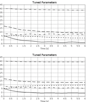
Figure 2.14: Tuning of the adaptive parameters in the lack of unknown disturbances:

with modified tuning without RFPT (upper chart), and modified tuning with RFPT(lower chart)[Θ₁: solid,Θ₂: dashed,Θ₃: dense dash,Θ₄: dash-dot, andΘ₅: dash-dot-dot lines]

Figure 2.15: The tracking error under unknown disturbances: with modified tuningwithout RFPT(upper chart), and modified tuningwith RFPT(lower chart)[q1: solid,q2: dashed,q3: dense dash lines]

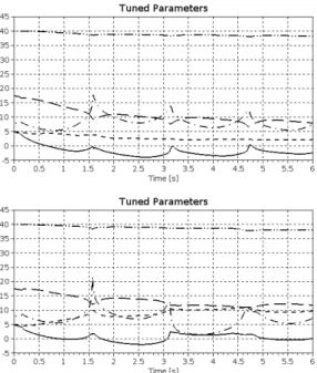
Figure 2.16 reveals that similar “abnormal” tuning-discrepancies occur in both cases, but the

(34)

RFPT-based method well compensates the simultaneous consequences of the disturbances and improper parameter tuning.

Figure 2.16: Tuning of the adaptive parameters under unknown disturbances: with modified tuningwithout RFPT(upper chart), and modified tuningwith RFPT(lower chart)[Θ₁: solid, Θ₂: dashed,Θ₃: dense dash,Θ₄: dash-dot, andΘ₅: dash-dot-dot lines]

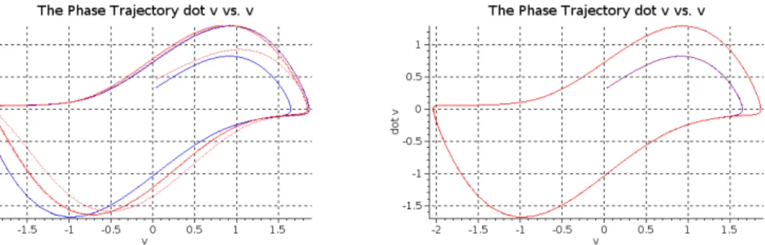
In this case important details are revealed by the phase trajectories (Fig. 2.17). Without using the RFPT-based adaptation more even and greater tracking errors are present. The RFPT reduces these errors in long sections, while in the problematic sections it generates significant changes in the phase space. Certain details can also be observed in the charts of trajectory tracking (Fig. 2.18). In Fig. 2.19 the operation of the RFPT-based method is illustrated: the realized (simulated)2^ndtime-derivative is in the close vicinity of the kinematically computed

“desired” value, i.e. the primary design intent, i.e. the realization of a kinemtically prescribed tracking error relaxation is successfully demonstrated.

(35)

Figure 2.17: The phase trajectories under unknown disturbances: with modified tuningwithout RFPT(upper chart), and modified tuningwith RFPT(lower chart)[q1: solid,q2: dashed, q3: dense dash lines]

Figure 2.18: The trajectory tracking under unknown disturbances: with modified tuning without RFPT (upper chart), and modified tuning with RFPT (lower chart)[q₁: solid, q₂: dashed,q₃: dense dash lines]

(36)

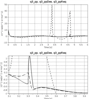
Figure 2.19: The second time-derivatives of generalized coordinateq₃ with modified tuning and RFPT-based adaptation (zoomed excerpt in the lower chart) [¨q₃ (realized): solid, q¨^Des₃ (“desired”): dashed,q¨₃^Req (adaptively deformed): dense dash lines]

(37)

2.5 Novel Tuning Method for the Modified Adaptive In- verse Dynamic Robot Controller (MAIDRC)

In this section I present that the SGFPT can also well coexist with the MAIDRC control design. I propose a novel, even simpler tuning method that also applies fixed-point transformation based tuning rule for parameter identification [A. 4].

2.5.1 Improvement in the MAIDRC control design

The theoretical considerations are validated by numerical simulations of the adaptive control of a 2 DoF (Degree of Freedom) paradigm. This approach uses the formal properties of the dyanamic model of the system under control as

H(q)¨q+h(q,q)˙ ≡Y(q,q,˙ q)Θ =¨ Q , (2.24) in whichH > 0the positive definite symmetric inertia matrix, qis the generalized coordi- nate of the system,Y(q,q,˙ q)¨ is precisely known on the basis of thekinematic modelof the controlled system, Q is the exerted generalized control forces, while Θis the array of the dynamic parameters that are only imprecisely known. Let the approximate values notated as H,ˆ ˆh, andΘ, respectively. The PID-typeˆ kinematic trajectory tracking error relaxationwas prescribed asq¨^Des= ¨q^{N om}+ 3Λ²(q^{N om}−q) + Λ³Rt

0 q^{N om}(ξ)−q(ξ)

dξ. For theadaptive deformationthe same function was used here, as in [A. 10]:

F(x)^def= atanh(tanh(x+D)/2) , h_i ^def= f(r_i)−r_i+1^Des ,

e_i ^def= _kh^hⁱ

ik ,

r_i+1 =G r_i, f(r_i), r^Des_i+1 def

= [F (Akh_ik+x_?)−x_?]e_i +r_i ,

(2.25)

whereF(x_?) = x_?, and the Frobenius norm is in use. The applied new type of function is detailed in section 4.2. Let the exerted control force calculated as

Q_n= ˆH(q_n) [r_n] + ˆh(q_n,q˙_n) , (2.26) that, according to (2.24), must be equal toH(q_n)¨q_n+h(q_n,q˙_n). By subtractingHˆq¨+ ˆhfrom both sides we get information on the actual modeling errors as