Fractional-Order Models for Biochemical Processes Eva-H. Dulf

(1)

Article

Fractional-Order Models for Biochemical Processes

Eva-H. Dulf^1,2 , Dan C. Vodnar³ , Alex Danku¹, Cristina-I. Muresan^1,* and Ovidiu Crisan^4,*

1 Faculty of Automation and Computer Science, Technical University of Cluj-Napoca, 400144 Cluj-Napoca, Romania; eva.dulf@aut.utcluj.ro (E.-H.D.); alex.danku@aut.utcluj.ro (A.D.)

2 Physiological Controls Research Center,Óbuda University, H-1034 Budapest, Hungary

3 Food Science and Technology Department, University of Agricultural Sciences and Veterinary Medicine Cluj-Napoca, 400372 Cluj-Napoca, Romania; dan.vodnar@usamvcluj.ro

4 Department of Organic Chemistry, Iuliu Hat,ieganu University of Medicine and Pharmacy, 400012 Cluj-Napoca, Romania

* Correspondence: Cristina.Muresan@aut.utcluj.ro (C.-I.M.); ocrisan@umfcluj.ro (O.C.)

Received: 22 February 2020; Accepted: 8 April 2020; Published: 10 April 2020 Abstract: Biochemical processes present complex mechanisms and can be described by various computational models. Complex systems present a variety of problems, especially the loss of intuitive understanding. The present work uses fractional-order calculus to obtain mathematical models for erythritol and mannitol synthesis. The obtained models are useful for both prediction and process optimization. The models present the complex behavior of the process due to the fractional order, without losing the physical meaning of gain and time constants. To validate each obtained model, the simulation results were compared with experimental data. In order to highlight the advantages of fractional-order models, comparisons with the corresponding integer-order models are presented.

Keywords: biochemical process; fractional order model; optimization

1. Introduction

Scientists have found that many diseases which affect the circulatory and the digestive systems are caused by the high intake of sugars. An initiative was taken by several countries in order to decrease the amount of sugar used in foods by using alternative natural sweeteners, such as mannitol and erythritol. It has been proven that natural sweeteners provide both a low glycemic index and a small number of calories.

Lactic acid bacteria (LAB) are known to produce erythritol and mannitol in dough preparations, hence they are being added to bakery products to add nutritional value and promote several positive health effects. Furthermore, since mannitol and erythritol are natural sweeteners, their use lowers the amount of sugar needed to prepare the products. One of the most used LAB isLactobacillus plantarum.

This bacterium is adaptable to other microorganisms and environments and is often used in food fermentation processes.Lactobacillus casei, also recognized for its adaptability, is used mainly in the dairy industry due to its capability to metabolize different carbohydrates. The difference between the two bacteria is thatL. plantarumhas a fast growth and its fermentation is anaerobic, whileL. caseiis characterized by aerobic fermentation and grows slowly.

The production of functional foods requires ingredients which are rich in nutrients (such as carbohydrates, vitamins, lipids, etc.). It has been proven by nutritionists that soybeans are an excellent source of most nutrients, and there have been reports that their active component (isoflavones) has positive effects on many diseases caused by a high consumption of sugar. For this reason, f soy flour can be introduced in wheat flour in order to increase the bioactive characteristics of the final bakery products.

Fractal Fract.2020,4, 12; doi:10.3390/fractalfract4020012 www.mdpi.com/journal/fractalfract

(2)

Fractal Fract.2020,4, 12 2 of 12

The primary cause of dental caries, obesity, type 2 diabetes, cancer, and cardiovascular diseases is the consumption of foods with a high sugar content [1,2]. To decrease the consumption of added and free sugars, taking into account the instructions by the World Health Organization (WHO), several countries are adopting regulations for lowering the sugar intake of the population, especially children [3]. The incorporation of alternative natural sweeteners (i.e., polyols), like mannitol or erythritol in bakery products, presents various favorable effects [4]. The digestion of these non-nutritive sweeteners is not entirely attainable by humans, and the majority is excreted unaltered in urine, providing a low source of calories and a low glycemic index [5].

Traditional food upgrading helps to enhance the nutritional values of foodstuffby providing several health-promoting effects [6]. Fermented foods frequently contain polyols, because they are the metabolic product of several starter cultures. The incorporation of LAB capable of producing mannitol or erythritol in dough preparations can contribute to the significant reduction of added sugars in bakery products [7]. L. plantarum, used in vegetable and other food fermentations, is a facultative heterofermentative bacterium and possesses competent adaptability to other microorganisms and environments. L. casei, also an adaptive bacterium mainly used in the dairy industry, is capable to metabolize different carbohydrates and has heterolactic and homolactic characteristics [8].L. plantarum grows faster with mainly anaerobic fermentation, whileL. caseigrows more slowly, and its fermentation is aerobic [9].

Soybean, of the Fabaceae family, is often used in the production of functional foods because it is rich in nutrients such as carbohydrates, lipids, proteins, minerals, vitamins and bioactive components such as isoflavones (30% daidzein and 60% genistein) [10]. Isoflavones possess many health-promoting properties, exerting positive effects against cancer, cardiovascular disease, hypercholesterolemia, osteoporosis, and atherosclerosis [11]. The integration of soy flour in wheat flour is advantageous nutritionally, and theβ-glucosidase enzyme from LAB can increase the aglycone content of dough by also increasing the bioactive and functional characteristics of bakery products [12].

Fractional calculus is a generalization of ordinary calculus which introduces derivatives and integrals of fractional order. Fractional calculus represents a very broad research field dealing with derivatives of arbitrary order [13]. Applications can be found in different research fields, ranging from systems engineering [14] to chemical and biochemical applications [15].

The goal of this paper was to optimize the mannitol and erythritol synthesis processes using different types of bacteria. To fulfil this objective, multiple models were created for each bacterial type. Second-order models were developed, which are widely used in technological process modelling.

For each dataset, fractional-order models were also developed, being recognized for their good phenomenological description [13–15]. Fractional-order models maintain the physical meaning of the gains and time constants, varying only the model order. The model validation was realized in comparison with experimental data. Using the best models, optimum process values were established.

The paper is structured in three parts. After this introduction, Section2discusses the materials and methods used to produce the results, which are presented in Section3. The work ends with concluding remarks.

2. Materials and Methods

The present research used lactic acid bacteria producing erythritol and mannitol on a vegetable substrate i.e., wheat flour and soybean (in different concentrations). The lactic bacteria used were L. plantarum and L. casei. Based on the obtained results, the optimization of the fermentation and composition of the substrate was pursued using the same bacteria together with the yeast Saccharomices cerevisiae. In each experiment, erythritol, mannitol, and secondary metabolites were quantified, following fermentation on the plant substrate. Erythritol and secondary metabolites were quantified using high-performance liquid chromatography (HPLC). The microorganisms were studied on 3 different doughs containing 10% soybean flour and 90% wheat flour, 5% soybean meal and 95% wheat flour, or 100% wheat flour. During lactic fermentation, the samples were taken at regular

(3)

intervals (0 h, 2 h, 4 h, 6 h, 8 h, 10 h, 24 h) from all the above-mentioned environments. In these samples, it was possible to determine the viability of microorganisms, their rate of multiplication, adaptation in the new environment, but also the content of the metabolites of interest for this research, i.e., erythritol and mannitol.

In order to optimize the production of erythritol and mannitol, two important aspects were considered: the microorganisms’ metabolic activity and the parameters of fermentation process.

The objective of the fermentation process was to favor the growth of L. plantarumandL. casei by using only the mentioned raw materials (wheat and soy flour). The final products obtained with the raw materials presented qualities which depended on the fermentation time, and most of them were associated with the metabolites synthesized during fermentation.

In recent years, a lot of work has been being carried out in physics and biophysics to create models for biological and complex processes. In many cases, linear differential equations provide highly successful models, but these models describe only the basis of many physiological systems. Many trials have been made using models with probabilistic, chaotic, and even fractal measures. Problems occur when the complexity of the model requires too much computational power or the obtained model is applicable using a narrow range of parameters. It is widely considered that fractional-order models can be applied on multiple scales not requiring multiple definitions of the model’s properties, thus reducing computations. A disadvantage of the fractional models is that some properties of differentiation are lost, which makes check-ups necessary to determine whether the obtained mathematical operations are allowed. Many papers have described successful models for different dynamic systems. The wide variety of applications extend from neural systems, for which Gaussian distribution and weighted summation of exponentials proved to provide incomplete explanations, to different bioengineering applications. Using fractional-order models, complex systems can be simulated with electrical systems containing capacitors and inductors.

The behavior of biotechnological systems has memory or aftereffects. If the output of a system at a certain time depends only on the input at that specific time, then such systems are said to be memoryless systems. On the other hand, if the system uses previous values of the input in order to determine the current value of the output, then such systems are considered systems with memory [13–15], which is the case of biotechnological systems. The modelling of these systems by fractional-order differential equations has more advantages than the classical integer-order mathematical modelling, in which such effects are neglected. Also, the fractional-order models are at least as stable as their integer-order counterparts [16–18]. It is also proven that in real-life situations, the created fractional-order mathematical models allow displaying some extra cases regarding the mathematical model equilibrium point stability region. For all these reasons, fractional-order mathematical models are more realistic and feasible [17–19].

The mathematical definition of the fractional-order model uses the Gamma function. For that equation, the Laplace transform is applied, giving the equation bellow [20]:

Ln t⁻^ko

= Γ(1−k)

s¹⁻^k , k<1 (1)

s^k⁻¹= ¹ Γ(k)Γ(1−k)

Z ^∞

0

a^k⁻¹

s+ada (2)

Equation (2) is obtained from Equation (1) by changing the order of integration betweenaandt.

Using the Stieltjes transform on Equation (2) gives the final form of the fractional derivative operator:

s^k= ¹

Γ(_k)Γ(₁⁻_k) Z ^∞

0

τ⁻^k τs τs+1

dτ

τ (3)

(4)

As a suitable mathematical model is essential for process optimization and prediction, the present research deals with an alternative tool, based on the use of fractional-order differential equations for biochemical processes identification, using experimental data. Matlab^® software (version R2019a, 1994–2020 The MathWorks, Inc., Natick, MA, USA) was used to perform the modeling, analyses, and plots. For fractional-order approximation, a toolbox for Matlab was used, namely, ninteger, a freely downloadable toolbox from the Internet [21].

As identification technique, a fully recurrent neural network with one hidden layer was used.

The cost function for training is the sum of mean squared errors:

CF= ¹ N

N

X

i=1

εiε^T_i = ¹ N

N

X

i=1

(yi−yˆi)(yi−yˆi)^T (4)

whereNis the number of training samples,yis the measured output, and ˆy is the output of the neural network.

As simulation toolbox, a modelling tool previously developed [22] was used.

3. Results

For the kinetics study of production, in each case, an integer-order model was developed using the Identification Toolbox from Matlab^®, having the form:

Hi(s) = ^k

(T₁s+1)(T₂s+1) ⁽⁵⁾ The experimental data, in all cases, suggested that an overdamped transfer function was suitable for modelling such processes. Additionally, a second-order model was selected for simplicity. In cases where this simple model was not suitable, a third-order model was developed:

Hi(s) = ^k

(T₁s+1)(T2s+1)(T3s+1) ⁽⁶⁾ The second stage of the research consisted in establishing fractional-order models in a form similar to transfer functions (5) or (6):

H f(s) = ^k

(_T₁_s^α+1)(_T₂_s^β+1) ⁽⁷⁾

H f(s) = ^k

(T1s^α+1)(T2s^β+1)(T3s^χ+1) ⁽⁸⁾ The integer- and fractional-order models have the same number of time constants,T1andT2for transfer function (5) and (7), andT₁,T_2,andT₃for transfer functions (6) and (8), and an additional gaink.

For the fractional-order transfer function (7) or (8), two or three supplementary model parameters were introduced, i.e., the fractional ordersα,β, andχIt was expected that using these extra model parameters, a better fit would be obtained, although the overall structure of the fractional-order model was maintained simple as in the integer-order case, with the same physical interpretation of time constants and gains.

3.1. Case 1: L. Plantarum

Using theL. plantarumbacterium, three experiments were made. The first one used 100% wheat flour. The following models were, obtained described by the integer-order transfer function (9) and the correspondent fractional-order transfer function (10).

Hi(s) = ^3.1969

(2.6s+1)(3s+1)(3s+1) ⁽⁹⁾

(5)

H f(_s) = ^3.1969

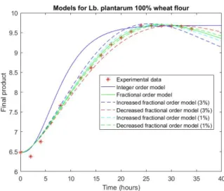
(23.4s^1.405+24.6s^1.85+8.6s³+1.295) ⁽¹⁰⁾ In Figure1, the behavior of the two transfer functions for the first set of experimental data can be seen. The fractional-order model (green line) followed the pattern of the experimental data (red dots). After 30 h, the model decreased slightly, which was not observed for the simpler model (blue line), considering its simple form. The mean squared error for the fractional-order model was 0.0048 and that for the integer-order model was 0.1207. The two dotted lines in Figure1represent similar fractional-order models with the same time constants, but their exponents are increased by 3% for the blue dotted line and decreased by 3% for the red dotted line. The intermediary orders are presented in green. The behavior of all fractional-order models was similar. Depending on the values chosen for the exponents, the model could reach its maximum value faster or slower. After 30 h, all three fractional systems started to decrease from their maximum value, a property which could be hardly found in integer-order models. The next figures contain the same elements and have been denoted with the same types of line and color.

Fractal Fract. 2020, 4, x FOR PEER REVIEW 5 of 13

presented in green. The behavior of all fractional-order models was similar. Depending on the values chosen for the exponents, the model could reach its maximum value faster or slower. After 30 h, all three fractional systems started to decrease from their maximum value, a property which could be hardly found in integer-order models. The next figures contain the same elements and have been denoted with the same types of line and color.

Figure 1. Comparison between simulated and experimental data for experiment 1 using Lactobacillus plantarum.

The next set of data used the same bacterium, but the flour mixture contained 95% wheat flour and 5% soy flour. The obtained models are transfer functions (11) and (12):

𝐻𝑖(𝑠) = 3.2553

(6.5𝑠 + 1)(6.5𝑠 + 1) (11)

𝐻𝑓(𝑠) = 3.2553

(42.5𝑠 ^. + 13𝑠 ^. + 1.045) (12)

In Figure 2 are presented the corresponding simulation results, for both integer- and fractional- order model. By comparing their behaviors and computing the mean squared error, it was concluded that the fractional-order model was more accurate than the simple, integer-order one. For the fractional-order model, the mean squared error was 0.0029, while for the integer-order model, it was 0.1516. In this case, the model represented by the red dotted line remained at its maximum value for longer, not decreasing for the entire simulation time.

Figure 2. Comparison between simulated and experimental data for experiment 2 using L. plantarum.

Figure 1. Comparison between simulated and experimental data for experiment 1 using Lactobacillus plantarum.

Hi(s) = ^3.2553

(6.5s+1)(6.5s+1) ⁽¹¹⁾

H f(s) = ^3.2553

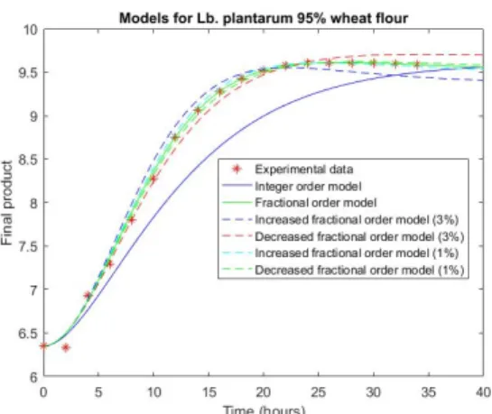
(42.5s^2.335+13s^1.13+1.045) ⁽¹²⁾ In Figure2are presented the corresponding simulation results, for both integer- and fractional-order model. By comparing their behaviors and computing the mean squared error, it was concluded that the fractional-order model was more accurate than the simple, integer-order one. For the fractional-order model, the mean squared error was 0.0029, while for the integer-order model, it was 0.1516. In this case, the model represented by the red dotted line remained at its maximum value for longer, not decreasing for the entire simulation time.

(6)

presented in green. The behavior of all fractional-order models was similar. Depending on the values chosen for the exponents, the model could reach its maximum value faster or slower. After 30 h, all three fractional systems started to decrease from their maximum value, a property which could be hardly found in integer-order models. The next figures contain the same elements and have been denoted with the same types of line and color.

Figure 1. Comparison between simulated and experimental data for experiment 1 using Lactobacillus plantarum.

𝐻𝑖(𝑠) = 3.2553

(6.5𝑠 + 1)(6.5𝑠 + 1) (11)

𝐻𝑓(𝑠) = 3.2553

(42.5𝑠 ^. + 13𝑠 ^. + 1.045) (12)

In Figure 2 are presented the corresponding simulation results, for both integer- and fractional- order model. By comparing their behaviors and computing the mean squared error, it was concluded that the fractional-order model was more accurate than the simple, integer-order one. For the fractional-order model, the mean squared error was 0.0029, while for the integer-order model, it was 0.1516. In this case, the model represented by the red dotted line remained at its maximum value for longer, not decreasing for the entire simulation time.

Figure 2.Comparison between simulated and experimental data for experiment 2 usingL. plantarum.

For the last experiment with this type of bacterium, the flour mixture contained 90% wheat flour and 10% soy flour. The developed models are presented in Equations (13) and (14):

Hi(_s) = ^3.2109

(2s+₁)(2s+₁)(2.6s+₁) ⁽¹³⁾

H f(s) = ^3.2109

(_10.4s^1.285+14.4s^1.45+6.6s³+1.15) ⁽¹⁴⁾ Figure3presents the corresponding experiment results for the first type of bacterium examined.

The models had similar behaviors as those observed in the first experiment, experiencing a decrease after a certain time, which with the simple model was more difficult to achieve. The mean squared error for the fractional model was 0.0758 and that for the integer-order model was 0.1628. The behavior of the fractional-order models was in this case similar to that of the first experiment. This similarity was observed in most of the following simulations.

For the last experiment with this type of bacterium, the flour mixture contained 90% wheat flour and 10% soy flour. The developed models are presented in Equations (13) and (14):

𝐻𝑖(𝑠) = 3.2109

(2𝑠 + 1)(2𝑠 + 1)(2.6𝑠 + 1) (13)

𝐻𝑓(𝑠) = 3.2109

(10.4𝑠^. + 14.4𝑠^. + 6.6𝑠 + 1.15) (14)

Figure 3 presents the corresponding experiment results for the first type of bacterium examined.

The models had similar behaviors as those observed in the first experiment, experiencing a decrease after a certain time, which with the simple model was more difficult to achieve. The mean squared error for the fractional model was 0.0758 and that for the integer-order model was 0.1628. The behavior of the fractional-order models was in this case similar to that of the first experiment. This similarity was observed in most of the following simulations.

3.2. Case 2: L. Casei

The next group of experiments used the L. casei bacterium and the same mixtures as a substrate.

The first models used the 100% wheat flour mixture:

𝐻𝑖(𝑠) = 3.781

(2.5𝑠 + 1)(3𝑠 + 1)(2.5𝑠 + 1) (15)

𝐻𝑓(𝑠) = 3.781

(18.75𝑠 ^. + 21.25𝑠 ^. + 8𝑠 ^. + 1.27) (16) As in the previous case, the fractional-order model was more accurate compared to the simple model. The errors were 0.0083 for the fractional-order model and 0.1879 for the integer-order model.

The comparative results are shown in Figure 4.

Figure 3.Comparison between simulated and experimental data for experiment 3 usingL. plantarum.

3.2. Case 2: L. Casei

The next group of experiments used theL. caseibacterium and the same mixtures as a substrate.

The first models used the 100% wheat flour mixture:

Hi(_s) = ^3.781

(2.5s+₁)(3s+₁)(2.5s+₁) ⁽¹⁵⁾

H f(s) = ^3.781

(_18.75s^1.36+_21.25s^1.8+_8s^2.5+_1.27) ⁽¹⁶⁾

(7)

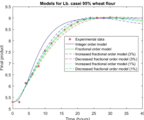
As in the previous case, the fractional-order model was more accurate compared to the simple model. The errors were 0.0083 for the fractional-order model and 0.1879 for the integer-order model.

The comparative results are shown in FigureFractal Fract. 2020, 4, x FOR PEER REVIEW 4. 7 of 13

Figure 4. Comparison between simulated and experimental data for experiment 1 using Lactobacillus casei.

The next model used a mixture of 95% wheat flour and 5% soy flour. In this case, the integer- and the fractional-order models obtained were:

𝐻𝑖(𝑠) = 3.6946

(2𝑠 + 1)(3𝑠 + 1)(3𝑠 + 1) (17)

𝐻𝑓(𝑠) = 3.6946

(12𝑠^. + 16𝑠 ^. + 7𝑠 ^. + 1.1) (18)

In this case, the mean squared errors for both models were small, i.e., 0.0056 for the fractional- order model and 0.0611 for the integer-order one. Both models behave in a similar manner. However, as it is also indicated in Figure 5, the fractional-order model approximated better the experimental data and thus represented a better choice.

Figure 5. Comparison between simulated and experimental data for experiment 2 using L. casei.

The last experiment used 90% wheat flour and 10% soy flour and produced the following results regarding the integer- and fractional-order models:

𝐻𝑖(𝑠) = 3.6385

(9𝑠 + 1)(9𝑠 + 1) (19)

𝐻𝑓(𝑠) = 3.6385

(81𝑠 ^. + 18𝑠 ^. + 1.29) (20)

Figure 4. Comparison between simulated and experimental data for experiment 1 using Lactobacillus casei.

Hi(s) = ^3.6946

(2s+1)(3s+1)(3s+1) ⁽¹⁷⁾ H f(s) = ^3.6946

(12s^1.16+16s^1.8+7s^2.5+1.1) ⁽¹⁸⁾ In this case, the mean squared errors for both models were small, i.e., 0.0056 for the fractional-order model and 0.0611 for the integer-order one. Both models behave in a similar manner. However, as it is also indicated in Figure5, the fractional-order model approximated better the experimental data and thus represented a better choice.

Figure 4. Comparison between simulated and experimental data for experiment 1 using Lactobacillus casei.

𝐻𝑖(𝑠) = 3.6946

(2𝑠 + 1)(3𝑠 + 1)(3𝑠 + 1) (17)

𝐻𝑓(𝑠) = 3.6946

(12𝑠 ^. + 16𝑠 ^. + 7𝑠 ^. + 1.1) (18)

In this case, the mean squared errors for both models were small, i.e., 0.0056 for the fractional- order model and 0.0611 for the integer-order one. Both models behave in a similar manner. However, as it is also indicated in Figure 5, the fractional-order model approximated better the experimental data and thus represented a better choice.

𝐻𝑖(𝑠) = 3.6385

(9𝑠 + 1)(9𝑠 + 1) (19)

𝐻𝑓(𝑠) = 3.6385

(81𝑠 ^. + 18𝑠 ^. + 1.29) (20)

Figure 5.Comparison between simulated and experimental data for experiment 2 usingL. casei.

Hi(s) = ^3.6385

(9s+1)(9s+1) ⁽¹⁹⁾

(8)

H f(s) = ^3.6385

(81s^2.25+18s^1.25+1.29) ⁽²⁰⁾ In the last experiment, the two models behave differently. The behavior of the fractional-order model was more accurate than that of the integer-order one. The error for the fractional-order model was 0.0034 and that for the classical model was 0.3829. The results are presented in Figure6.

In the last experiment, the two models behave differently. The behavior of the fractional-order model was more accurate than that of the integer-order one. The error for the fractional-order model was 0.0034 and that for the classical model was 0.3829. The results are presented in Figure 6.

3.3. Case 3: L. Casei + L. Plantarum

The following experiments used contain both types of bacteria. The first set of data were obtained using 100% wheat flour. The following integer-order and fractional-order models were obtained:

𝐻𝑖(𝑠) = 3.13

(6.5𝑠 + 1)(6.5𝑠 + 1) (21)

𝐻𝑓(𝑠) = 3.13

(42.25𝑠^. + 13𝑠^. + 1.06) (22)

In this particular case, the mean squared error for the fractional-order model was 0.0042, while that for the integer-order model was significantly larger, equal to 0.1523. The comparative simulation results against the experimental data are presented in Figure 7.

Figure 7. Comparison between simulated and experimental data for experiment 1 using both types of bacteria.

The next experiment used 5% soy flour and 95% wheat flour. Two models were determined here, and the results are indicated in Figure 8. The two models are:

Figure 6.Comparison between simulated and experimental data for experiment 3 usingL. casei.

3.3. Case 3: L. Casei+L. Plantarum

Hi(s) = ^3.13

(6.5s+1)(6.5s+1) ⁽²¹⁾

H f(s) = ^3.13

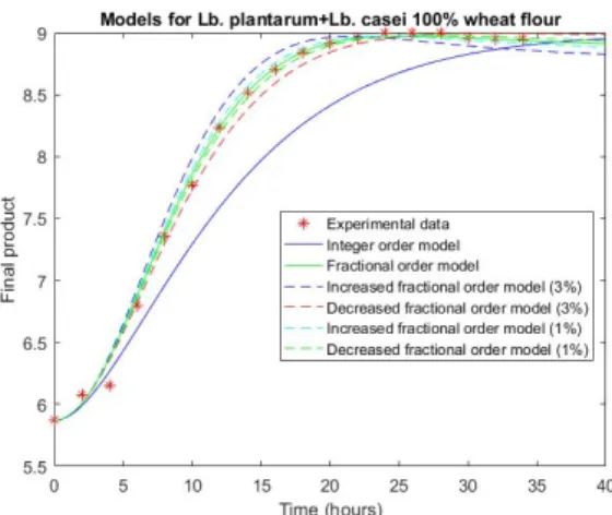
(42.25s^2.375+13s^1.14+1.06) ⁽²²⁾ In this particular case, the mean squared error for the fractional-order model was 0.0042, while that for the integer-order model was significantly larger, equal to 0.1523. The comparative simulation results against the experimental data are presented in Figure7.

In the last experiment, the two models behave differently. The behavior of the fractional-order model was more accurate than that of the integer-order one. The error for the fractional-order model was 0.0034 and that for the classical model was 0.3829. The results are presented in Figure 6.

3.3. Case 3: L. Casei + L. Plantarum

𝐻𝑖(𝑠) = 3.13

(6.5𝑠 + 1)(6.5𝑠 + 1) (21)

𝐻𝑓(𝑠) = 3.13

(42.25𝑠^. + 13𝑠^. + 1.06) (22)

In this particular case, the mean squared error for the fractional-order model was 0.0042, while that for the integer-order model was significantly larger, equal to 0.1523. The comparative simulation results against the experimental data are presented in Figure 7.

The next experiment used 5% soy flour and 95% wheat flour. Two models were determined here, and the results are indicated in Figure 8. The two models are:

Figure 7.Comparison between simulated and experimental data for experiment 1 using both types of bacteria.

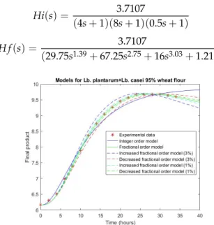
The next experiment used 5% soy flour and 95% wheat flour. Two models were determined here, and the results are indicated in Figure8. The two models are:

(9)

Hi(s) = ^3.7107

(4s+1)(8s+1)(0.5s+1) ⁽²³⁾

H f(s) = ^3.7107

(29.75s^1.39+67.25s^2.75+16s^3.03+1.215) ⁽²⁴⁾

𝐻𝑖(𝑠) = 3.7107

(4𝑠 + 1)(8𝑠 + 1)(0.5𝑠 + 1) (23)

𝐻𝑓(𝑠) = 3.7107

(29.75𝑠^. + 67.25𝑠^. + 16𝑠 ^. + 1.215) (24)

In this case, in the first part of the simulation, both models had small errors. However, the fractional-order model was able to follow the decreasing slope of the experimental results, unlike the integer-order model. The mean squared errors were 0.001 in the case of the fractional-order model and 0.0159 for the integer-order one.

The last models created used 10% soy flour and 90% wheat flour. The following transfer functions were obtained:

𝐻𝑖(𝑠) = 3.9740

(6.3𝑠 + 1)(3.7𝑠 + 1)(0.7𝑠 + 1) (25)

𝐻𝑓(𝑠) = 3.9740

(16.317𝑠 ^. + 30.31𝑠 ^. + 10.7𝑠^. + 1.1) (26) In the last case, the mean squared errors of the two models were higher than those measured previously. The error of the fractional-order model was 0.1469, while that of the other model was 0.2676. In this case, the simple form of the integer-order model failed to cover all experimental points, as indicated in Figure 9.

All these results are summarized in Table 1.

In this case, in the first part of the simulation, both models had small errors. However, the fractional-order model was able to follow the decreasing slope of the experimental results, unlike the integer-order model. The mean squared errors were 0.001 in the case of the fractional-order model and 0.0159 for the integer-order one.

The last models created used 10% soy flour and 90% wheat flour. The following transfer functions were obtained:

Hi(_s) = ^3.9740

(6.3s+₁)(3.7s+₁)(0.7s+₁) ⁽²⁵⁾

H f(s) = ^3.9740

(16.317s^1.27+30.31s^2.9+10.7s^2.6+1.1) ⁽²⁶⁾ In the last case, the mean squared errors of the two models were higher than those measured previously. The error of the fractional-order model was 0.1469, while that of the other model was 0.2676.

In this case, the simple form of the integer-order model failed to cover all experimental points, as indicated in Figure9.

All these results are summarized in TableFractal Fract. 2020, 4, x FOR PEER REVIEW 1. 10 of 13

Table 1. Mean square errors for each experiment.

Experiment 100% Wheat 95% Wheat 90% Wheat

Experiment with L. plantarum

0.0048 for Fractional 0.1207 for Integer

Experiment with L. casei

Experiment with L. casei + L. plantarum

The well-known disadvantage of fractional-order models is complexity. The integer-order approximation which gives proper results is very important for simulation and process optimization.

For this reason, different approximations of fractional orders were applied for every identified fractional-order model, and the execution time for a step response was measured. The results are presented in Table 2. It can be concluded that the computational costs are not relevant for these models.

(10)

Table 1.Mean square errors for each experiment.

Experiment 100% Wheat 95% Wheat 90% Wheat

Experiment with L. plantarum

0.0758 for Fractional 0.1628 for Integer Experiment withL. casei 0.0083 for Fractional

0.1879 for Integer

0.0034 for Fractional 0.3829 for Integer Experiment withL. casei

+L. plantarum

The well-known disadvantage of fractional-order models is complexity. The integer-order approximation which gives proper results is very important for simulation and process optimization.

For this reason, different approximations of fractional orders were applied for every identified fractional-order model, and the execution time for a step response was measured. The results are presented in Table2. It can be concluded that the computational costs are not relevant for these models.

Table 2.Algorithm execution time depending on the fractional-order approximationn.

Experiment Approximation Ordern

100% Wheat Execution Time

L. plantarum

2 0.630840 0.553088 0.622764

4 0.628559 0.561806 0.619775

6 0.666731 0.548033 0.622020

8 0.651018 0.571900 0.657854

10 0.638888 0.619697 0.623748

L. casei

2 0.633670 0.672707 0.553984

4 0.674323 0.624525 0.563766

6 0.617245 0.645090 0.560314

8 0.669795 0.611367 0.571462

10 0.627036 0.795508 0.633211

L. casei+ L. plantarum

2 0.564722 0.685146 0.634549

4 0.693730 0.619232 0.624525

6 0.573994 0.664748 0.645380

8 0.605419 0.621814 0.668827

10 0.567797 0.618991 0.621872

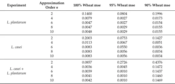
For computational cost evaluation, each fractional-order model was approximated with integer-order elements havingn=2, 4, 6, 8, 10 elements. The results are presented in Table3.

Table 3.Algorithm mean squared error (mse) for different fractional-order approximationsn.

Experiment Approximation

Ordern 100% Wheat mse 95% Wheat mse 90% Wheat mse

L. plantarum

2 0.1400 0.0804 0.1996

4 0.0079 0.0027 0.0173

6 0.0047 0.0027 0.0154

8 0.0047 0.0029 0.0155

10 0.0048 0.0029 0.0155

L. casei

2 0.2003 0.0753 0.1427

4 0.0113 0.0067 0.0051

6 0.0083 0.0550 0.0036

8 0.0083 0.0056 0.0034

10 0.0083 0.0056 0.0034

L. casei+ L. plantarum

2 0.0857 0.2726 0.4376

4 0.0036 0.0045 0.1472

6 0.0039 0.0010 0.1437

8 0.0041 0.0010 0.1460

10 0.0042 0.0010 0.1469

(11)

It can be concluded that by using a larger approximation number, the error decreased, but after n=6, the differences were too small or smaller than 10⁻⁴. Naturally, the downside of using a larger value is the more complex form of the approximated transfer function, but this does not affect the execution time of the algorithm, as presented in Table2.

4. Conclusions

In order to optimize the chosen biochemical process and predict different evolutions, mathematical modelling was realized. In the present work, integer-order and fractional-order models were presented. The classical integer-order models were established with the specific toolbox in Matlab^®. The fractional-order models were developed using artificial intelligence. The results proved the superiority of the models created with fractional-order tools in comparison with classical integer-order ones.

Author Contributions: Conceptualization, E.-H.D.; methodology, C.-I.M.; software, A.D.; validation, O.C.;

data curation, D.C.V.; writing—original draft preparation, E.-H.D. and A.D.; writing—review and editing, C.-I.M.

All authors have read and agreed to the published version of the manuscript.

Funding:This research was funded by a grant of the Romanian National Authority for Scientific Research, CNDI–

UEFISCDI, project number PN-III-P1-1.2-PCCDI2017-0056, contract 2PCCDI/2018. D.E.H. was funded by the Hungarian Academy of Science, Janos Bolyai Grant (BO/00313/17) and theÚNKP-19-4-OE-64 New National Excellence Program of the Ministry for Innovation and Technology.

Conflicts of Interest:The authors declare no conflict of interest.

References

1. Bailey, R.L.; Fulgoni, V.L.; Cowan, A.; Gaine, P. Sources of Added Sugars in Young Children, Adolescents, and Adults with Low and High Intakes of Added Sugars.Nutrients2018,10, 102. [CrossRef] [PubMed]

2. Sadeghirad, B.; Johnston, B.C. The Scientific Basis of Guideline Recommendations on Sugar Intake.Ann. Intern.

Med.2017,166, 257–267. [CrossRef] [PubMed]

3. Braesco, V.A.; Sluik, D.; Privet, L.; Kok, F.J.; Moreno, L.A. A review of total & added sugar intakes and dietary sources in Europe.Nutr. J.2017,16, 6.

4. Luo, X.; Arcot, J.; Gill, T.; Louie, J.C.Y.; Rangan, A. A review of food reformulation of baked products to reduce added sugar intake.Trends Food Sci. Technol.2019,86, 412–425. [CrossRef]

5. Lin, S.-D.; Mau, J.; Lin, L.-Y.; Lee, C.-C.; Chiou, S.-Y. Effect of Erythritol on Quality Characteristics of Reduced-Calorie Danish Cookies.J. Food Qual.2010,33, 14–26. [CrossRef]

6. Ronda, F. Effects of polyols and nondigestible oligosaccharides on the quality of sugar-free sponge cakes.

Food Chem.2005,90, 549–555. [CrossRef]

7. Rice, T.; Zannini, E.; Arendt, E.K.; Coffey, A. A review of polyols—Biotechnological production, food applications, regulation, labeling and health effects. Crit. Rev. Food Sci. Nutr. 2019,6, 1–18. [CrossRef]

[PubMed]

8. Stefanovic, E.; Fitzgerald, G.; McAuliffe, O. Advances in the genomics and metabolomics of dairy lactobacilli:

A review.Food Microbiol.2017,61, 33–49. [CrossRef] [PubMed]

9. Păucean, A.; Vodnar, D.C.; Socaci, S.A.; Socaciu, C. Carbohydrate metabolic conversions to lactic acid and volatile derivatives, as influenced by Lactobacillus plantarum ATCC 8014 and Lactobacillus casei ATCC 393 efficiency during in vitro and sourdough fermentation.Eur. Food Res. Technol.2013,237, 679–689. [CrossRef]

10. Hu, C.; Wong, W.-T.; Wu, R.; Lai, W. Biochemistry and use of soybean isoflavones in functional food development.Crit. Rev. Food Sci. Nutr.2019,7, 1–15. [CrossRef] [PubMed]

11. Faraj, A.; Vasanthan, T. Soybean Isoflavones: Effects of Processing and Health Benefits.Food Rev. Int.2004, 20, 51–75. [CrossRef]

12. Zhang, B.; Yang, Z.; Huang, W.; Omedi, J.O.; Wang, F.; Zou, Q.; Zheng, J. Isoflavone aglycones enrichment in soybean sourdough bread fermented by lactic acid bacteria strains isolated from traditional Qu starters:

Effects on in vitro gastrointestinal digestion, nutritional, and baking properties. Cereal Chem. J.2018,96, 129–141. [CrossRef]

13. Monje, C.A.; Chen, Y.Q.; Vinagre, B.M.; Xue, D.; Feliu, V.Fractional-Order Systems and Controls; Chapter 4;

Springer-Verlag: London, UK, 2010.

(12)

14. Dulf, E.H.; Dulf, F.V.; Pop, C.I. Fractional model of the cryogenic (¹³C) isotope separation column.Chem.

Eng. Commun.2015,202, 1600–1606. [CrossRef]

15. Dulf, E.H.; Muresan, C.I.; Unguresan, M.L. Modeling the (¹⁵N) isotope separation column.J. Math. Chem.

2014,52, 115–131. [CrossRef]

16. Atangana, A.; Gómez-Aguilar, J. Numerical approximation of Riemann-Liouville definition of fractional derivative: From Riemann-Liouville to Atangana-Baleanu. Numer. Methods Partial. Differ. Equ.2017,34, 1502–1523. [CrossRef]

17. Saad, K.M.; Gómez-Aguilar, J. Analysis of reaction–diffusion system via a new fractional derivative with non-singular kernel.Phys. A Stat. Mech. Appl.2018,509, 703–716. [CrossRef]

18. Gómez-Aguilar, J.; Morales, V.; Taneco, M. Analytical solution of the time fractional diffusion equation and fractional convection-diffusion equation.Rev. Mex. Física2018,65, 82–88. [CrossRef]

19. Atangana, A.; Gómez-Aguilar, J. Fractional derivatives with no-index law property: Application to chaos and statistics.Chaos Solitons Fractals2018,114, 516–535. [CrossRef]

20. Magin, R.L. Fractional calculus models of complex dynamics in biological tissues.Comput. Math. Appl.2010, 59, 1586–1593. [CrossRef]

21. Duarte, V.; José, S.D.C. Ninteger: A Non-Integer Control Toolbox for MatLab. In Proceedings of the 1st IFAC Workshop on Fractional Differentiation and Its Applications, Bordeaux, France, 19–21 July 2004.

22. Dulf, E.; Vodnar, D.C.; Dulf, F.V. Modeling tool using neural networks for l(+)-lactic acid production by pellet-form Rhizopus oryzae NRRL 395 on biodiesel crude glycerol. Chem. Cent. J.2018, 12, 124–129.

[CrossRef] [PubMed]

©2020 by the authors. Licensee MDPI, Basel, Switzerland. This article is an open access article distributed under the terms and conditions of the Creative Commons Attribution (CC BY) license (http://creativecommons.org/licenses/by/4.0/).