Vol. 20 (2019), No. 1, pp. 193–208 DOI: 10.18514/MMN.2019.2768
SIGN-CONSTANCY OF GREEN’S FUNCTIONS FOR TWO-POINT IMPULSIVE BOUNDARY VALUE PROBLEMS
A. DOMOSHNITSKY AND IU. MIZGIREVA Received 01 December, 2018
Abstract. We consider the following second order impulsive differential equation with delays 8
ˆ<
ˆ:
.Lx/.t /x00.t /CPp
jD1aj.t /x0.t j.t //CPp
jD1bj.t /x.t j.t //Df .t /;
t2Œ0; !;
x.tk/Dkx.tk 0/; x0.tk/Dıkx0.tk 0/; kD1; 2; :::; r:
In this paper we obtain sufficient conditions of nonpositivity of Green’s functions for impuls- ive differential equation. All results are formulated in the form of theorems about differential inequalities. It should be noted that the sign-constancy of the coefficientsbj.t /was assumed in all the literature devoted to impulsive functional differential equations. One of the main purposes of this work is to propose a technique allowing us to avoid these assumptions.
2010Mathematics Subject Classification: 34K10; 34K45
Keywords: second order impulsive differential equations, boundary value problems, sign-constancy of Green’s functions
1. INTRODUCTION
Impulsive differential equations have attracted an attention of a number of recog- nized mathematicians and have applications in many spheres of science from physics, biology, medicine to economical studies. The following well-known books can be noted in this context [14,17–19]. In the book [3], the concept of the general theory of functional differential equations was presented. On the basis of this concept nonos- cillation for the first order functional differential equations was considered in [4], where positivity of the Cauchy and Green’s functions of the periodic problem was firstly studied. A concept of nonoscillation for the first order differential equations is also considered in the book [1]. The positivity of Green’s function of one- and two-point boundary value problems for functional differential impulsive equations was studied in [2,5–8,10–13,15]. It should be noted that the sign-constancy of the coefficientsbj.t /was assumed in all the results for impulsive functional differential
This paper is part of the second author’s Ph.D. thesis which is being carried out in the Department of Mathematics at Ariel University.
c 2019 Miskolc University Press
equations. One of the main purposes of this work is to propose a technique allowing us to avoid these assumptions.
Let us consider the following impulsive equations:
.Lx/.t /x00.t /C
p
X
jD1
aj.t /x0.t j.t //C
p
X
jD1
bj.t /x.t j.t //Df .t /; t2Œ0; !;
(1.1) x.tk/Dkx.tk 0/; x0.tk/Dıkx0.tk 0/; kD1; 2; :::; r;
0Dt0< t1< t2< ::: < tr< trC1D!; (1.2)
x./D0; x0./D0; < 0; (1.3)
wheref,aj,bj: Œ0; !!Rare summable functions and j,j: Œ0; !!Œ0;C1/ are measurable functions forj D1; 2; :::; p,pandr are natural numbers,k andık are real positive numbers.
LetD.t1; t2; :::; tr/be a space of functionsx:Œ0; !!Rsuch that their derivative x0.t / is absolutely continuous on every interval t 2Œti; tiC1/, i D0; 1; :::; r, x00 2 L1, we assume also that there exist the finite limits x.ti 0/Dlimt!ti x.t /and x0.ti 0/Dlimt!ti x0.t /and condition (1.2) is satisfied at pointsti .i D0; 1; :::; r/.
As a solutionxwe understand a functionx2D.t1; t2; :::; tr/satisfying (1.1)-(1.3).
There is not many works on sign-constancy of Green’s functions of second-order impulsive boundary value problems. We can note only the results of [5–8,16] where these problems are considered. In these papers the coefficientsbj.t /were assumed to be nonpositive. Using approaches of these papers, we obtain the results on sign- constancy of Green’s functions to impulsive two-point boundary value problems without sign assumption on the coefficientsbj.t /. Our results are presented in the form of algebraic inequalities, establishing the smallness of the coefficients aj.t /, jbj.t /j,j D1; :::; p,t2Œ0; !.
2. PRELIMINARIES
For equation (1.1)-(1.3) we consider the following variants of boundary condi- tions:
x.0/D0; x.!/D0; (2.1)
x0.0/D0; x.!/D0; (2.2)
x.0/D0; x0.!/D0; (2.3)
x0.0/D0; x0.!/D0: (2.4)
General solution of the equation (1.1)-(1.3) can be represented in the form [4]:
x.t /D1.t /x.0/CC.t; 0/x0.0/C Z t
0
C.t; s/f .s/ds; (2.5) where
1.t /is a solution of the homogeneous equation .Lx/.t /x00.t /C
p
X
jD1
aj.t /x0.t j.t //C
p
X
jD1
bj.t /x.t j.t //D0; t2Œ0; !;
(2.6) x.tk/Dkx.tk 0/; x0.tk/Dıkx0.tk 0/; kD1; 2; :::; r;
0Dt0< t1< t2< ::: < tr< trC1D!; (2.7)
x./D0; x0./D0; < 0; (2.8)
with the initial conditionsx.0/D1,x0.0/D0.
C.t; s/, called the Cauchy function of the equation (2.6)-(2.8), is the solution of the equation
.Lsx/.t /x00.t /C
p
X
jD1
aj.t /x0.t j.t //C
p
X
jD1
bj.t /x.t j.t //D0; t2Œs; !;
(2.9) x.tk/Dkx.tk 0/; x0.tk/Dıkx0.tk 0/; kDm; :::; r;
0Dt0< t1< t2< ::: < tr< trC1D!; (2.10) wheremis a number, such thattm 1< stm,
x./D0; x0./D0; < s; (2.11)
satisfying the initial conditionsC.s; s/D0,Ct0.s; s/D1andC.t; s/D0for t < s.
If the boundary value problem (1.1)-(1.3), (2.i),iD1; 4is uniquely solvable, then its solution can be represented as
x.t /D Z !
0
Gi.t; s/f .s/ds; i D1; 4; (2.12) whereGi.t; s/is Green’s function of the problem (1.1)-(1.3), (2.i) respectively [5].
Using general representation of the solution (2.5), the following formulas for Green’s functions can be obtained:
G1.t; s/DC.t; s/ C.t; 0/C.!; s/
C.!; 0/; (2.13)
G2.t; s/DC.t; s/ C.!; s/1.t /
1.!/; (2.14)
G3.t; s/DC.t; s/ C.t; 0/Ct0.!; s/
Ct0.!; 0/; (2.15)
G4.t; s/DC.t; s/ Ct0.!; s/1.t /
10.!/: (2.16)
Below the following definition will be used.
Definition 1. We callŒ0; !a semi-nonoscillation interval of (2.6)-(2.8), if every nontrivial solution having zero of derivative does not have zero on this interval.
3. SIGN-CONSTANCY OFGREEN’S FUNCTIONS FORbj.t /0
Denote G.t; s/ the Green’s function of the problem (1.1)-(1.3) with boundary conditions
x./D0; x0./D0: (3.1)
In the paper [5], the following theorem has been proven for the problems (1.1)- (1.3), (2.i).
Lemma 1. Assume that the following conditions are fulfilled:
(1) bj.t /0,j D1; :::; p,t2Œ0; !.
(2) The Cauchy functionC1.t; s/of the first order impulsive equation y0.t /C
p
X
jD1
aj.t /y.t j.t //D0; t2Œ0; !;
y.tk/Dıky.tk 0/; kD1; 2; :::; r;
y./D0; < 0;
(3.2)
is positive for0st!.
(3) Green’s functionG.t; s/of the problem (1.1)-(1.3),(3.1) is nonnegative for t; s2Œ0; for every0 < < !.
(4) Œ0; !is a semi-nonoscilation interval of.Lx/.t /D0.
Then Green’s functionsGi.t; s/,i D1; 3are nonpositive fort; s2Œ0; !and under the additional conditionPp
jD1bj.t /Œ0;!.t j.t //60,t2Œ0; !, where Œ0;!.t /D
1; t2Œ0; !;
0; t62Œ0; !; (3.3)
G4.t; s/0fort; s2Œ0; !.
Using the results of [9] (see Theorems 4.1 and 4.2 from [9]), it is easy to see, that if aj.t /0, j D1; :::; p, t 2Œ0; !, then the assumption4) follows from the rest 3 assumptions of Lemma1, so we can exclude it and rewrite Theorem1in the following form.
Theorem 1. Assume that the following conditions are fulfilled:
(1) aj.t /0,bj.t /0,j D1; :::; p,t2Œ0; !.
(2) The Cauchy functionC1.t; s/of the first order equation (3.2) is positive for 0st !.
(3) Green’s functionG.t; s/of the problem (1.1)-(1.3),(3.1) is nonnegative for t; s2Œ0; for every0 < < !.
Then Green’s functionsGi.t; s/,i D1; 3are nonpositive fort; s2Œ0; !and under the additional conditionPp
jD1bj.t /Œ0;!.t j.t //60,t2Œ0; !, Green’s function G4.t; s/0fort; s2Œ0; !.
In Theorem1we have assumed that the Cauchy functionC1.t; s/of the first order impulsive equation (3.2) is positive. In the lemma below, we will formulate the results of [4] on the conditions of positivity of Cauchy function of the first order impulsive differential equation
y0.t /Ca1.t / y.t 1.t //D0; t2Œ0; !;
y.tk/Dıky.tk 0/; kD1; 2; :::; r;
y./D0; < 0:
(3.4) Lemma 2. Let0 < ıj < 1forjD1; :::; rand the following condition be fulfilled
1ClnB.t /
e
Z t m.t /
aC.s/ds; (3.5)
where B.t /DQ
j2Dtıj, Dt D fi Wti 2Œt 1.t /; t g, aC.t /Dmaxfa1.t /; 0gand m.t /Dmaxft 1.t /; 0g. Then Cauchy function of the first order impulsive differen- tial equation (3.4) is positive.
In the case ofp > 1the following sufficient condition proven in [4] can be used.
Lemma 3. Letaj.t /0forj D1; :::; p,0 < ık1forkD1; :::; rand Z !
0 p
X
jD1
aj.s/ds <
r
Y
kD1
ık; (3.6)
then Cauchy function of the first order impulsive differential equation (3.2) is positive.
In the next section we will consider an auxiliary impulsive boundary value prob- lem, which will provide the conditions of nonnegativity of Green’s functionG.t; s/.
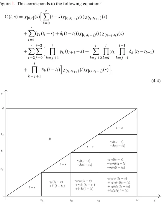
4. AUXILIARY BOUNDARY VALUE PROBLEMx00.t /D´.t / Let us consider the following equation:
x00.t /D´.t /; t2Œ0; !; (4.1)
x.tk/Dkx.tk 0/; x0.tk/Dıkx0.tk 0/; kD1; 2; :::; r; (4.2)
x./D0; x0./D0; < 0: (4.3)
Denote byC .t; s/N the Cauchy function of the equation (4.1)-(4.3). According to [6], Cauchy function for this impulsive equation has the form, represented on the
Figure1. This corresponds to the following equation:
C .t; s/N DŒ0;t .s/hXr
iD0
.t s/Œti;tiC1/.t /Œti;tiC1/.s/
C
r
X
iD1
.i.ti s/Cıi.t ti//Œti;tiC1/.t /Œti 1;ti/.s/
C
r
X
iD2 i 2
X
jD0
h Yi
kDjC1
k.tjC1 s/C
i
X
lDjC2 i
Y
kDl
k l 1
Y
kDjC1
ık.tl tl 1/
C
i
Y
kDjC1
ık.t ti/i
Œti;tiC1/.t /Œtj;tjC1/.s/i :
(4.4)
s
t1 t t1
t2
t2
t3
t3
ω ω
t−s
t−s
t−s
t−s
γ3(t3−s) +δ3(t−t3)
γ2(t2−s) +δ2(t−t2)
γ1(t1−s) +δ1(t−t1)
γ2γ1(t1−s) +γ2δ1(t2−t1) +δ2δ1(t−t2)
γ3γ2(t2−s) +γ3δ2(t3−t2) +δ3δ2(t−t3)
γ3γ2γ1(t1−s) +γ3γ2δ1(t2−t1) +γ3δ2δ1(t3−t2) +δ3δ2δ1(t−t3) 0
FIGURE1. The Cauchy function of impulsive equation (4.1) - (4.3).
Let us build now the Green’s function G.t; s/N of the problem (4.1)-(4.3) with boundary conditions
x.!/D0; x0.!/D0: (4.5)
The solution of this boundary value problem will be of the following form:
x.t /D Z !
0
hC .t; s/N C 1.t / 1.!/
hCNt0.!; s/
CNt0.!; 0/C .!; 0/N C .!; s/N i C .t; 0/N
CNt0.!; 0/
i
´.s/ds;
(4.6)
with the corresponding Green’s function G.t; s/N D NC .t; s/C 1.t /
1.!/
hCNt0.!; s/
CNt0.!; 0/C .!; 0/N C .!; s/N i C .t; 0/N
CNt0.!; 0/; (4.7) where
1.t /D
(1; t2Œ0; t1/;
Qr
kD1k; t 2Œtk; tkC1/: (4.8) See the graphical representation of Green’s functionG.t; s/N on the Figure2.
s
t1 t t1
t2
t2
t3
t3
ω ω
−(t−s)
−(t−s)
−(t−s)
−(t−s)
1 δ3(t3−t) +γ13(s−t3)
0
1 δ2δ3(t2−t) +γ1
2δ3(t3−t2) +γ1
2γ3(s−t3)
(t1−t)
δ1δ2δ3+(tγ12−tδ2δ13) + +(tγ3−t2)
1γ2δ3+(s−tγ 3)
1γ2γ3
(t1−t)
δ1δ2 +(tγ2−t1δ21)+(s−tγ1γ22)
1 δ2(t2−t) +γ12(s−t2)
1 δ1(t1−t) +γ11(s−t1)
FIGURE2. The Green’s function of impulsive equation (4.1) - (4.3), (4.5).
Theorem 2. If aj.t /0, bj.t /0 for j D1; p, 0 < k 1, 0 < ık 1 for kD1; r, and if the condition
! Qr
kD1ıkess sup
t2Œ0;!
p
X
jD1
jaj.t /j
C!
r
X
iD1
ti ti 1
Qr
kDiıkQi kD1k
iC ! tr
Qr kD1k
! ess sup
t2Œ0;!
p
X
jD1
jbj.t /j< 1
(4.9)
is satisfied, then Green’s functionG.t; s/of the (1.1)-(1.3),(4.5) is nonnegative.
Proof. We can rewrite equation (1.1)-(1.3) in the form
´.t /C
p
X
jD1
aj.t / Z !
0
GN0t t j.t /; s
Œ0;! t j.t /
´.s/ds
C
p
X
jD1
bj.t / Z !
0
G tN j.t /; s
Œ0;! t j.t /
´.s/dsDf .t /:
(4.10)
Denote the operatorK:L1!L1as follows:
.K´/.s/D Z !
0
h
p
X
jD1
aj.t /GNt0 t j.t /; s
Œ0;! t j.t /
p
X
jD1
bj.t /G tN j.t /; s
Œ0;! t j.t /i
´.s/ds:
(4.11)
Foraj.t /0,bj.t /0,j D1; :::; p, the operatorK: L1!L1is positive. If the spectral radius .K/ < 1, then the solution of (4.10) can be represented in the form:
´D.I K/ 1f D 2 4
1
X
jD0
Kj 3
5f: (4.12)
The solutionx.t /of the boundary value problem (1.1)-(1.3),(4.5) can be written in the form:
xD 0
@GN
1
X
jD0
Kj 1
Af; (4.13)
whereGN P1
jD0Kj is Green’s operator for (1.1)-(1.3) with boundary conditions (4.5).
From nonnegativity of Green’s functionG.t; s/N and positivity of operatorK:L1! L1it follows that Green’s functionG.t; s/for (1.1)-(1.3),(4.5) is nonnegative.
Now let us find the conditions that the spectral radius of the operatorK: L1! L1is less than one. It is satisfied, when
ess sup
t2Œ0;!
p
X
jD1
jaj.t /jess sup
t2Œ0;!
Z !
0 j NG0t.t; s/jds Cess sup
t2Œ0;!
p
X
jD1
jbj.t /jess sup
t2Œ0;!
Z !
0 j NG.t; s/jds < 1:
(4.14)
If0 < k1,0 < ık 1forkD1; r, then:
ess sup
t;s2Œ0;!Œ0;!j NG.t; s/j D
r
X
iD1
ti ti 1
Qr
kDiıkQi kD1k
iC ! tr
Qr
kD1k; (4.15) ess sup
t;s2Œ0;!Œ0;!
j NGt0.t; s/j D 1 Qr
kD1ık
: (4.16)
Thus, the spectral radius.K/ < 1, if0 < k 1,0 < ık1forkD1; r and
! Qr
kD1ık ess sup
t2Œ0;!
p
X
jD1
jaj.t /j
C!
r
X
iD1
ti ti 1
Qr
kDiıkQi
kD1kiC ! tr
Qr kD1k
! ess sup
t2Œ0;!
p
X
jD1
jbj.t /j< 1:
(4.17)
Example1. Let us consider the following differential equation
x00.t /Ca1.t /x0.t 1.t //Cb1.t /x.t 1.t //Df .t /; t2Œ0; 3; (4.18) with impulses (1.2), where
t1D1; 1D0:9; ı1D0:5;
t2D1:5; 2D0:6; ı2D0:7;
t3D2:5; 3D0:8; ı3D0:4;
(4.19) anda1.t /0,b1.t /0.
For an auxiliary differential equation
x00.t /D´.t /; t2Œ0; 3; (4.20)
with impulses (1.2), (4.19) and boundary conditions
x.3/D0; x0.3/D0; (4.21)
we constructed Green’s functionG.t; s/. It is represented on the FigureN 3 and its derivativeGNt0.t; s/- on the Figure4.
t 0.0 0.5
1.0 1.5
2.0 2.5
3.0 s
0.0 0.5
1.0 1.5 2.0 2.53.0 G(t,s)
0 5 10
0 2 4 6 8 10 12 14
FIGURE3. G.t; s/N of (4.20), (4.19), (4.21).
Calculating maximum values ofj NG.t; s/jandj NG0t.t; s/jint; s2Œ0; 3Œ0; 3, we obtain:
ess sup
t;s2Œ0;3Œ0;3j NG.t; s/j D14:914; (4.22) ess sup
t;s2Œ0;3Œ0;3
j NG0t.t; s/j D7:143: (4.23) According to Theorem2, for our example, we obtain the following condition of positivity of Green’s functionG.t; s/:
21:429 ess sup
t2Œ0;3ja1.t /j C 44:742 ess sup
t2Œ0;3jb1.t /j< 1: (4.24)
t 0.0 0.5
1.0 1.5
2.0 2.5
3.0 s
0.0 0.5
1.0 1.5 2.0 2.53.0 G'(t,s)
−6
−4
−2 0
−7
−6
−5
−4
−3
−2
−1 0
FIGURE4. GN0t.t; s/of (4.20), (4.19), (4.21).
5. SIGN-CONSTANCY OFGREEN’S FUNCTIONS FOR THE CASE WHENbj.t /CAN CHANGE SIGN
For the case whenbj.t /, j D1; :::; p, changes sign, there can be considered an auxiliary differential equation:
.L x/.t /x00.t /C
p
X
jD1
aj.t /x0.t j.t //C
p
X
jD1
bj .t /x.t j.t //D´.t /; t2Œ0; !;
(5.1) x.tk/Dkx.tk 0/; x0.tk/Dıkx0.tk 0/; kD1; 2; :::; r;
0Dt0< t1< t2< ::: < tr< trC1D!; (5.2)
x./D0; x0./D0; < 0; (5.3)
where
bj .t /D
bj.t /; bj.t /0;
0; bj.t / > 0: (5.4)
The solution for the boundary value problems (5.1)-(5.3), (2.i) can be written in the form
x.t /D Gi ´ .t /
Z ! 0
Gi .t; s/´.s/ds; i D1; 4: (5.5) The given equation (1.1) can be written in the form:
.Lx/.t /D.L x/.t /C
p
X
jD1
bjC.t /x.t j.t //Df .t /; (5.6) where
bjC.t /D
bj.t /; bj.t / > 0;
0; bj.t /0: (5.7)
After the substitution (5.5) into (5.6) we obtain
´.t /C
p
X
jD1
bjC.t / Z !
0
Gi t j.t /; s
Œ0;! t j.t /
´.s/dsDf .t /; iD1; 4:
(5.8) Define the integral operatorsKiWL1!L1for each type of boundary conditions (iD1; 4) by the equality:
.Ki´/.t /D
p
X
jD1
bjC.t / Z !
0
Gi t j.t /; s
Œ0;! t j.t /
´.s/ds: (5.9) Its spectral radius can be denoted by.Ki/.
We propose an assertion about nonpositivity of Green’s function of (1.1)-(1.3), (2.i) without an assumptionbj.t /0,j D1; :::; p. For this case we can reformulate Theorem1as follows.
Theorem 3. Assume that the following conditions are fulfilled:
(1) aj.t /0,j D1; :::; p,t2Œ0; !.
(2) The Cauchy functionC1.t; s/of the first order equation (3.2) is positive for 0st !.
(3) Green’s functionG.t; s/of the problem (5.1)-(5.3),(3.1) is nonnegative for t; s2Œ0; for every0 < < !.
(4) .Ki/ < 1.
Then Green’s functionsGi.t; s/,iD1; 3are nonpositive fort; s2Œ0; !and under the additional conditionPp
jD1bj .t /Œ0;!.t j.t //60, t 2Œ0; !, Green’s function G4.t; s/0fort; s2Œ0; !.
Proof. The conditions (1)-(3) of Theorem3 correspond to all the conditions of Theorem1, so they guarantee that Green’s functionsGi .t; s/,iD1; 4, are nonposit- ive.
We have assumed above, in equation (5.7), thatbjC.t /0. Together with the fact thatGi .t; s/0, according to Corollary1, it implies that the operatorsKi,i D1; 4, are positive.
If the condition.Ki/ < 1holds, then the equation (5.8) can be written as follow- ing:
´D.I Ki/ 1f D 2 4
1
X
jD0
Kij 3
5f: (5.10)
It follows fromGi .t; s/0that all operatorsKij are positive and, consequently, for this caseP1
jD0Kij 0.
The solution x.t /of the given boundary value problem (1.1)-(1.3), (2.i) can be written in the form:
xD 0
@Gi
1
X
jD0
Kij 1
Af; (5.11)
where Green’s operator for the problem (1.1)-(1.3), (2.i) is GiDGi
1
X
jD0
Kij; (5.12)
which is nonpositive when the condition.Ki/ < 1holds.
For the case whenbj.t /can change sign, we can also use the following form of Theorem1.
Corollary 1. Assume that the following conditions are fulfilled:
(1) 0 < k1,0 < ık1forkD1; r andaj.t /0,j D1; :::; p,t2Œ0; !.
(2) The condition (3.6) is fulfilled.
(3) The inequality
p
X
jD1
aj.t /GN0t t j.t /; s
Œ0;! t j.t /
p
X
jD1
bj.t /G tN j.t /; s
Œ0;! t j.t / 0
(5.13)
is fulfilled fort2Œ0; !.
(4) The condition (4.17) is fulfilled.
Then Green’s functionsGi.t; s/,i D1; 3are nonpositive fort; s2Œ0; !and under the additional conditionPp
jD1bj.t /Œ0;!.t j.t //60,t2Œ0; !, Green’s function G4.t; s/0fort; s2Œ0; !.
Example 2. Let us consider the same equation as in Example1, where a1.t /D 0:015tC0:005,b1.t /D0:005t 0:005(so,b1.t /changes sign at the pointtD1), 1.t /D0:5,1.t /D0:5.
x00.t /C.0:015tC0:005/x0.t 0:5/C.0:005t 0:005/x.t 0:5/Df .t /; t2Œ0; 3;
(5.14) with impulses (1.2), where
t1D1; 1D0:9; ı1D0:5;
t2D1:5; 2D0:6; ı2D0:7;
t3D2:5; 3D0:8; ı3D0:4:
(5.15) Let us verify if the condition (5.13) is satisfied. Denote
M.t; s/D .0:015tC0:005/GNt0.t 0:5; s/ Œ0;3.t 0:5/
.0:005t 0:005/G .tN 0:5; s/ Œ0;3.t 0:5/ : (5.16) The form of functionM.t; s/, for our example, is shown on Figure5. It is easy to see that the functionM.t; s/0fort; s2Œ0; 3Œ0; 3. Thus, the condition3) of Corollary1is fulfilled.
Now let us verify the condition (4.17). It is equivalent to the condition:
ess sup
t;s2Œ0;3Œ0;3
Z 3 0
M.t; s/ds < 1; (5.17)
or
ess sup
t;s2Œ0;3Œ0;3
M.t; s/ < 1
3: (5.18)
For our example, we can calculate ess sup
t;s2Œ0;3Œ0;3
M.t; s/D0:18: (5.19)
Substituting this into the equation (5.18), we can obtain:0:18 < 13. Thus, the condi- tion4) of Corollary1is fulfilled.
Let us use Lemma3to check the condition2) of Corollary1. We can calculate:
Z 3 0
.0:015tC0:005/dtD0:0825;
3
Y
kD1
ıkD0:14:
We obtain0:0825 < 0:14, thus, the condition2) of Corollary1holds. So, all the con- ditions of Corollary1are fulfilled. It means that, for our example, Green’s functions Gi.t; s/,iD1; 4are nonpositive.
t 0.0 0.5
1.0 1.5
2.0 2.5
3.0 s
0.0 0.5
1.0 1.5 2.0 2.53.0 M(t,s)
0.00 0.05 0.10 0.15
0.00 0.05 0.10 0.15
FIGURE5. M.t; s/.
REFERENCES
[1] R. P. Agarwal, L. Berezansky, E. Braverman, and A. Domoshnitsky, Nonoscillation Theory of Functional Differential Equations with Applications. New York: Springer, 2012. doi:
10.1007/978-1-4614-3455-9.
[2] R. P. Agarwal and D. O’Regan, “Multiple Nonnegative Solutions for Second Order Impulsive Differential Equations.”Applied Mathematics and Computation, vol. 114, no. 1, pp. 51–59, 2000, doi:10.1016/S0096-3003(99)00074-0.
[3] N. V. Azbelev, V. P. Maksimov, and L. F. Rakhmatullina,Introduction to the Theory of Functional Differential Equations: Methods and Applications. New York: Hindawi, 2007.
[4] A. Domoshnitsky and M. Drakhlin, “Nonoscillation of First Order Impulsive Differential Equa- tions With Delay.”Journal of Mathematical Analysis and Applications, vol. 206, no. 1, pp. 254–
269, 1997.
[5] A. Domoshnitsky and G. Landsman, “Semi-nonoscillation Intervals in the Analysis of Sign Con- stancy of Green’s Functions of Dirichlet, Neumann and Focal Impulsive Problems.”Advances in Difference Equations, vol. 81, no. 1, 2017, doi:10.1186/s13662-017-1134-1.
[6] A. Domoshnitsky, G. Landsman, and S. Yanetz, “About Sign-constancy of Green’s Functions for Impulsive Second Order Delay Equations.”Opuscula Mathematica, vol. 34, no. 2, pp. 339–362, 2014, doi:10.7494/OpMath.2014.34.2.339.
[7] A. Domoshnitsky, G. Landsman, and S. Yanetz, “About Sign-constancy of Green’s Functions of One-point Problem for Impulsive Second Order Delay Equations.”Functional Differential Equa- tions, vol. 21, no. 1–2, pp. 3–15, 2014.
[8] A. Domoshnitsky, G. Landsman, and S. Yanetz, “About Sign-constancy of Green’s Function of a Two-point Problem for Impulsive Second Order Delay Equations.”Electronic Journal of Qualit- ative Theory of Differential Equations, vol. 9, pp. 1–16, 2016.
[9] A. Domoshnitsky, I. Mizgireva, and V. Raichik, “Semi-nonoscillation Intervals and Sign- constancy of Green’s Functions of Two-point Impulsive Boundary Value Problems.”Submitted to Ukrainian Mathematical Journal, 2018.
[10] M. Feng and D. Xie, “Multiple Positive Solutions of Multi-point Boundary Value Problem for Second-order Impulsive Differential Equations.”Journal of Mathematical Analysis and Applica- tions, vol. 223, no. 1, pp. 438–448, 2009.
[11] L. Hu, L. Liu, and Y. Wu, “Positive Solutions of Nonlinear Singular Two-point Boundary Value Problems for Second-order Impulsive Differential Equations.”Nonlinear Analysis: Theory, Meth- ods & Applications, vol. 69, no. 11, pp. 3774–3789, 2008, doi:10.1016/j.na.2007.10.012.
[12] T. Jankowsky, “Positive Solutions to Second Order Four-point Boundary Value Problems for Im- pulsive Differential Equations.”Applied Mathematics and Computation, vol. 202, no. 2, pp. 550–
561, 2008.
[13] D. Jiang and X. Lin, “Multiple Positive Solutions of Dirichlet Boundary Value Problems for Second Order Impulsive Differential Equations.”Journal of Mathematical Analysis and Applica- tions, vol. 321, no. 2, pp. 501–514, 2006.
[14] V. Lakshmikantham, D. Bainov, and P.S.Simeonov,Theory of Impulsive Differential Equations.
Singapore: World Scientific, 1989. doi:10.1142/0906.
[15] E. Lee and Y. Lee, “Multiple Positive Solutions of Singular Two Point Boundary Value Problems for Second Order Impulsive Differential Equations.”Applied Mathematics and Computation, vol.
158, no. 3, pp. 745–759, 2004.
[16] I. Mizgireva, “On Positivity of Green’s Functions of Two-point Impulsive Problems.”Submitted to Functional Differential Equations (accepted), vol. 24, no. 3–4, 2018.
[17] S. G. Pandit and S. G. Deo,Differential Systems Involving Impulses. Berlin: Springer-Verlag, 1982. doi:10.1007/BFb0067476.
[18] A. M. Samoilenko and N. A. Perestyuk,Impulsive Differential Equations. Singapore: World Scientific, 1995. doi:10.1142/2892.
[19] S. G. Zavalishchin and A. N. Sesekin, Dynamic Impulse Systems: Theory and Applications.
Springer Netherlands, 1997. doi:10.1007/978-94-015-8893-5.
Authors’ addresses
A. Domoshnitsky
Department of Mathematics, Ariel University, Israel E-mail address:adom@ariel.ac.il
Iu. Mizgireva
Department of Mathematics, Ariel University, Israel E-mail address:julia.mizgireva@gmail.com