ABS-Based Direct Method for Solving Complex Systems of Linear Equations

Article

ABS-Based Direct Method for Solving Complex Systems of Linear Equations

József Abaffy¹and Szabina Fodor^2,*

Citation: Abaffy, J.; Fodor, S.

ABS-Based Direct Method for Solving Complex Systems of Linear Equations.Mathematics2021,9, 2527.

https://doi.org/10.3390/math9192527

Academic Editors: Lorentz Jäntschi and Daniela Ros,ca

Received: 24 August 2021 Accepted: 3 October 2021 Published: 8 October 2021

Publisher’s Note:MDPI stays neutral with regard to jurisdictional claims in published maps and institutional affil- iations.

Copyright: © 2021 by the authors.

Licensee MDPI, Basel, Switzerland.

This article is an open access article distributed under the terms and conditions of the Creative Commons Attribution (CC BY) license (https://

creativecommons.org/licenses/by/

4.0/).

1 Institute of Applied Mathematics, Óbuda University, Bécsi út 96/b, 1034 Budapest, Hungary;

jozsef.abaffy@uni-obuda.hu

2 Department of Computer Science, Corvinus University of Budapest, F˝ovám tér 13-15, 1093 Budapest, Hungary

* Correspondence: szabina.fodor@uni-corvinus.hu; Tel.: +36-1-482-7468

Abstract:Efficient solution of linear systems of equations is one of the central topics of numerical computation. Linear systems with complex coefficients arise from various physics and quantum chemistry problems. In this paper, we propose a novel ABS-based algorithm, which is able to solve complex systems of linear equations. Theoretical analysis is given to highlight the basic features of our new algorithm. Four variants of our algorithm were also implemented and intensively tested on randomly generated full and sparse matrices and real-life problems. The results of numerical experiments reveal that our ABS-based algorithm is able to compute the solution with high accuracy.

The performance of our algorithm was compared with a commercially available software, Matlab’s mldivide(\) algorithm. Our algorithm outperformed the Matlab algorithm in most cases in terms of computational accuracy. These results expand the practical usefulness of our algorithm.

Keywords:complex linear system; direct method; ABS class of methods

1. Introduction

The problem of solving systems of linear equations plays a central role in diverse scientific fields such as signal processing, economics, computer science, and physics [1–5].

Often the problems arising from areas of practical life result in a system of equations with real coefficients, but there are important applications that lead to the following complex linear systems:

Ax=b, whereA∈C^m,n,x∈Cⁿandb∈C^m. (1) Partial differential equations modelling dissipative processes usually involve complex coefficient functions or complex boundary conditions [6]. Other applications leading to complex linear systems include the discretization of time-dependent Schrödinger equa- tions with implicit differential equations [7–9], inverse scattering problems, underwater acoustics, eddy current calculations [10], diffuse optical tomography [11], numerical calcu- lations in quantum chromodynamics and numerical conformal mapping [12]. There are several methods to solve complex systems of linear equations. Moreover, a complex linear system withnunknowns can be reformulated to a linear system of equations with 2nreal coefficients [13].

There are two basic popular approaches in solving complex linear systems of equations.

The first one is when the preconditioned classical conjugate gradient method is used to solve the system of equations [14–16]. In most of these cases, the algorithms often do not work with the original general, i.e., non-Hermitian Acoefficient matrix, but with a modified Hermitian positive definite normal equations

A^HAx=A^Hb, whereA^His the conjugate transpose of theAmatrix. (2)

Mathematics2021,9, 2527. https://doi.org/10.3390/math9192527 https://www.mdpi.com/journal/mathematics

The second popular approach is to solve usually non-symmetric linear systems of equa- tions using one of the generalized CG methods [17,18], such as GMRES ([19] pp. 164–185) or other approaches based on the Arnoldi or the Lanczos biconjugate algorithms. These approaches generate an orthogonal basis for the Krylov subspaces associated withAand an initial vectorv1. The usual way to obtain an approximation to the exact solution of (1) from this basis is to force a biconjugate gradient condition. In both cases, the resulting iterative methods tend to converge relatively slowly.

Mainly, two factors influence the practical usability of a method: the accuracy of the solutions and the computation cost of the method. There are two main classes of techniques for solving linear systems of equations: iterative and direct methods.

Iterative solvers are generally faster on large-scale problems, while direct ones give more accurate results. Not surprisingly, iterative methods have come to the fore in solving complex linear systems of equations and many new algorithms have been published in recent decades [20–22]. However, the robustness and the speed of the convergence of iterative algorithms significantly depend on the condition number of the coefficient ma- trices. To avoid convergence problems, robust preconditioners need to be used. In some cases, problem-specific preconditioners are highly effective, but they are often difficult to parallelize on modern high performance computing (HPC) platforms [23]. Moreover, Koric et al. [24] revealed that no iterative preconditioned solver combination could cor- rectly solve the highly ill-conditioned systems of equations. Therefore, researchers often have to compromise between accuracy of the solutions and computational effort. Direct solvers typically do not have these limitations but require much more computational power to execute. Thus, today’s high performance solutions such as parallel computing frameworks, may provide new possibilities for direct algorithms and they can be more suitable choices to ill-conditioned problems.

In this paper, we present a new ABS-based direct method that can solve large-scale problems. The ABS class of methods was originally introduced by Abaffy, Broyden and Spedicato (1984) developed to solve linear systems of equations where coefficients of the equations are real numbers [25]. These algorithms can also be used for various other purposes such as solving non-linear systems of equations or optimization problems [26–28].

ABS-based algorithms can be easily and effectively parallelised [29,30] which underlines the practical usefulness of these algorithms.

The remainder of this paper is organized as follows. In Section2, we present our new scaled complex ABS algorithm, which can solve complex linear systems of equations and we prove some of its basic features. We also show a special choice of parameters of our algorithm, which ensures that the search vectors (pi) areA^HAconjugate. We provide a detailed numerical analysis of four variants of our algorithm in Section3. Section4contains concluding remarks and a brief description of our plans on the application of the outcomes of this work.

2. The Scaled Complex ABS (scABS) Algorithm

In this section, we present our new ABS-based algorithm (scABS) that can solve systems of complex linear problems. Instead of the original system (1) let us consider the following scaled complex system of linear equations

V^HAx=V^Hb, whereV∈C^m,nis an arbitrary, non-singular matrix. (3) Note that the systems (1) and (3) are equivalent. Thus, if we want our algorithm to solve the original unscaled system of Equation (1), then by choosing the scaling matrix as the unit matrix we obtain the desired formulas and values. The sole role of the scaling matrixVis to provide significant flexibility to the algorithm [25] which allows us to reduce the computational inaccuracy [31] and also to reduce the computational complexity of the algorithm [27].

It is also of interest to note that our scaled complex ABS algorithm defines not one single algorithm, but a class of variants. Each particular variant is determined by the choice

of the parametersH₁,v_i,z_i,w_i. These variants have different properties, e.g., by choosing H₁ = Iunit matrix, v_i = AH_i^Hz_i, andw_ito be a multiple of z_i, the ABS algorithm is a reformulation of the QR algorithm, as we will discuss in Section2.2.

The state of the complex system of linear equations is checked by the variable si =HiA^Hvi. An important property of our algorithm is that si is zero if, and only if, the current row of matrix A is a linear combination of the previous rows. It depends on the value of the right-hand side whether our system is then a linear combination of the previous equations or even incompatible with them. We use the value ofx_ito distinguish between the two cases, namely whether it solves theithequation or not. If it does, we sim- ply skip the equation (xi+1=xi,Hi+1= Hi), otherwise, we stop the algorithm. The state of the system is stored in thei f lagvariable. Ifi f lagis zero, then neither linear dependency nor incompatibility is detected in the algorithm. If the value ofi f lagis positive, then a number of linearly dependent equations are found. If the value ofi f lagis negative then the−i f lagthequation is incompatible with the previous ones.

H1was selected to be a unit matrix for the sake of simplicity. However,H1could theoretically be any arbitrary unimodular nonsingular matrix provided thatH1∈C^n,n. 2.1. Basic Properties of the Scaled Complex ABS Algorithm

We consider some fundamental properties of theHigenerated by the scaled complex ABS (scABS) algorithm (Algorithm 1).

Theorem 1. Given the A^Hv₁,..., A^Hvm∈Cⁿvectors and the H₁∈C^n,narbitrary nonsingular matrix, consider the sequence of matrices H2, . . . ,H_m+1generated by (6). The following relations are true for i=2, . . . ,m+1:

HiA^Hvj=0, 1≤j<i. (4)

Proof. We proceed by induction. Fori=2, the theorem is true since H2=H₁−^H1A

Hv₁∗w₁^HH₁

wf₁ w₁^HH₁A^Hv₁.

H₂A^Hv₁=H₁A^Hv₁− ^H1A

Hv₁∗w^H₁H₁

wf₁ w^H₁H₁A^Hv₁∗A^Hv₁

=H₁A^Hv₁− ^H1A

Hv1∗w^H₁H1A^Hv1

wf1

w₁^HH₁A^Hv₁

=H1A^Hv1− ^H1A

Hv1∗w_f1

wf₁ =0.

Assuming that the theorem is true up toi<m, we prove it fori+1.

Hi+1=Hi−^HiA

Hvi∗w^H_i Hi

we_i w^H_i HiA^Hvi

Hi+1A^Hvj=HiA^Hvj− ^HiA

Hvi∗w_i^HHi

we_i w_i^HHiA^Hvi∗A^Hvj

=H_iA^Hv_j− ^HiA

Hv_i∗w_i^HH_iA^Hv_j

we_i w_i^HH_iA^Hv_i

=HiA^Hvj− ^HiA

Hvi∗w_ei

we_i =0.

Algorithm 1:Scaled complex ABS (scABS) algorithm.

Input:Setx₁∈C^n,H1= I∈C^n,nwhereIis the unit matrix,i=1, andi f lag=0.

Output:Solution to (3)x_i ∈Cⁿ, if the solution exists, otherwise the−i f lagth equation incompatible with the previous ones.

while(i≤m) and (i f lag≥0)do

Compute the scalarτ_i=v^H_i ri ∈Cand the vectorsi =HiA^Hvi, where r_i =Ax_i−b.

if(s_i=0) and (τ_i=0) and (i<m)then

/* The ith equation linearly depends on the previous ones. */

pi=0, xi+1=xi, Hi+1=_Hi, i f lag=i f lag+_1.

else if(si=0) and (τi =0) and (i=m)then xmis the solution.

else if(s_i=0) and (τ_i 6=0)then

/* The ith equation is incompatible with the previous ones. */

i f lag=−i.

else

Compute the search directionp_i

pi =H_i^Hzi, (5)

wherezi ∈Cⁿis arbitrary with the conditionz^H_i HiA^Hvi6=0.

xi+1=xi−α_ipi. Let introduce the notationαe_ias the denominator ofα_i

αe_i =v_i^HAp_i∗v_i^HAp_i,

wherev^H_i Ap_iis the complex conjugate ofv_i^HAp_ivector. Therefore,αe_iis a real number and the step sizeα_iis given by

α_i= ^τi

αe_i ∗v^H_i Ap_i. Update the projection matrix. Compute

Hi+1= Hi− ^HiA

Hvi∗w_i^HHi

wei w_i^HHiA^Hvi, (6) where we use the notionwe_ias denominator ofw_i.w_i ∈Cⁿis arbitrary with the condition

we_i=w_i^HH_iA^Hv_i∗w^H_i H_iA^Hv_i 6=0.

i=i+1

Remark 1. The null space of complex projection matrices Null(Hi) =A^Hv1,A^Hv2, . . . ,A^Hvi−1

follows immediately from Theorem1and it means that Hm+1=0

Remark 2. H_iA^Hv_icomputed by the scABS algorithm is zero only if A^Hv_iis a linear combination of A^Hv₁,A^Hv₂, . . . ,A^Hvi−1.

Remark 3. The scaled complex ABS algorithm is well defined.

Theorem 2. Consider the matrices H_igenerated by (6) with the starting H₁is nonsingular. For i=1, . . . ,m+1and1≤ j≤i the following relations are true:

HiH₁⁻¹Hj =Hi, (7)

H_jH₁⁻¹H_i =H_i. (8)

Proof. We only prove (7) since the proof for (8) is similar. We proceed by induction. For i=1,H1H₁⁻¹H1=H1is trivially true. Assuming now that (7) is true up to the indexi, we have to prove thatH_i+1H₁⁻¹H_j= H_i+1.

Forj=i+1, we have Hi+1H₁⁻¹Hi+1= (Hi−^HiA

Hv1∗w_i^HHi

we_i w_i^HHiA^Hvi)H₁⁻¹

∗(Hi− ^HiA

Hv_i∗w_i^HH_i

wei w^H_i HiA^Hvi)

= HiH₁⁻¹Hi−^HiA

Hvi∗w^H_i HiH₁⁻¹Hi

we_i w^H_i HiA^Hvi

− ^HiH

−1

1 H_iA^Hv_i∗w_i^HH_i wei

w_i^HH_iA^Hv_i

+ ^HiA

Hvi∗w_i^HHi

we_i w_i^HHiA^HviH₁⁻¹∗^HiA

Hvi∗w_i^HHi

we_i w_i^HHiA^Hvi

= H_iH₁⁻¹H_i−2∗ ^HiA

Hv_i∗w_i^HH_iH₁⁻¹H_i wei

w_i^HH_iA^Hv_i+ HiA^Hvi∗w^H_i Hi

we_i H₁⁻¹∗^HiA

Hvi∗w_i^HHi

we_i (w^H_i HiA^Hvi)²

= H_i−2∗^HiA

Hv_i∗w^H_i H_i wei

w^H_i H_iA^Hv_i

+ ^HiA

Hv_i∗w_ei∗w_i^HH_i

wei2 w_i^HH_iA^Hv_i

= H_i− ^HiA

Hv_i∗w_i^HH_i

we_i w_i^HH_iA^Hv_i=H_i+1. Forj<i+_{1, we have}

H_i+1H₁⁻¹H_j= (H_i− ^HiA

Hv1∗w^H_i H_i

we_i w^H_i H_iA^Hv_i)H₁⁻¹H_j

=Hi− ^HiA

Hv1∗w_i^HHi

wei w_i^HHiA^Hvi=Hi+1

again by the induction.

Remark 4. If H1is the unit matrix then Theorem2implies that Himatrices are idempotent, i.e., HiHi=Hi.

Remark 5. The H_iH_i = H_i feature of our algorithm enables further potential improvement in computational accuracy of the scaled complex ABS algorithm. We have recently published that the reprojection of real ABS algorithms, i.e., using p_i=H_i^H(H_i^Hz_i) projection vectors instead of pi=H_i^Hzi, enhances the precision of numerical calculation [30,31], which expands the practical usefulness of our algorithms.

Theorem 3. Any vector y∈Cⁿthat solves the first i equations of (3) can be formulated as

y=xi+1+H_i+1^H s (9)

where s is a vector inC^n.

Proof. Decomposey∈C^nasy=x_i+1+y⁺. Asysolves the firstiequations,

A^Hvjy=b^Hvj =A^Hvjxi+1+A^Hvjy⁺, where 1≤j≤i. (10) Thus,A^Hv_jy⁺ = 0 for 1≤ j ≤ iwhich means thaty⁺⊥{A^Hv₁, ..,A^Hv_i} = ⊥Null (H_i+1), soy⁺=H_i+1^H rwherer∈Cⁿaccording to the properties of the scaled complex ABS algorithm. Soy⁺ =H_i+1^H rwherer∈Cⁿaccording to the properties of ABS.

y⁺ =H_i+1^H r=H_i+1^H ·H_i+1^H r=H_i+1^H y⁺wherey⁺ ∈C^{n. (11)}

Remark 6. Referring to the proofs of the original ABS algorithm [26], it can be shown that, for simplicity, assuming that the A matrix is full rank, L_i=V_i^HA_iP_iis a nonsingular lower triangular matrix where P_i = (p₁, . . . ,p_i), V_i = (v₁, . . . ,v_i)and A_i = (a₁^H, . . . ,a^H_i )the transpose of the rows of the matrix A. If i=m, then the following semifactorization of the inverse can be obtained:

A⁻¹=PL⁻¹V^H, where P=Pm, and V =Vm. (12) This semi-factorization of the inverse of the A matrix may provide an opportunity to develop an ABS-based preconditioner to accelerate various Krylov subspace methods. For several choices of the matrix V, the matrix L is diagonal, hence formula (12) gives an explicit factorization of the inverse of the coefficient matrix A.

Remark 7. Examining the properties of the scaled complex ABS algorithm in terms of practical usability, we have already mentioned in Remark4that the idempotent property of the H_imatrix can be used to increase the computational accuracy of our algorithm by reprojection stepwise. Broyden showed [32] that the computation error in the solution is reduced up to2orders in _kH^kATvik2

iA^Tv_ik₂ for the real ABS algorithm. If the projection vectors (p_i) are re-projected with an additional computational cost, i.e., p_i = H_i^Tz_i = H_i^TH_i^Tz_i, a more accurate result can be obtained due to the cancellation errors in computational accuracy [33,34]. Interestingly, our preliminary results showed that the scABS algorithm has similar properties. Increasing accuracy in this way will result in a significant increase in computational costs. One solution to speed up the algorithm may be to parallelize the processes. In a recent paper [30], we found that for a real ABS algorithm, parallelization yielded a significant gain in computational speed.

2.2. Special Choice of the Scaling Vector

We consider the following choice of the scaling vector:

vi =Api. (13)

This selection of the scaling vector has many beneficial features such as

• the scaling vectors defined by (13) are mutually orthogonal, i.e., v_i^Hvj =0 fori>jandv_i^Hvi 6=0.

• the search vectorspiareA^HAconjugate ifAis square and nonsingular matrix.

• the algorithm generates an implicit factorization ofAinto the product of an orthogonal and an upper triangular matrix ifw_iis a multiple ofz_iandH₁=I(unit matrix). The algorithm with these selections can be considered as an alternative method of the classic QR factorization.

• by the choice of H₁ = I, z_i = w_i = e_i, the required number of multiplication is

11

6n³+O(n²).

The above statements about of the oscABS algorithm (Algorithm2) can be easily verified based on the proofs of Theorem 8.11, Theorem 8.16 and Theorem 8.18 in [25].

Algorithm 2:Orthogonally scaled complex ABS (oscABS) algorithm.

Input:Setx₁∈C^n,H1=I∈C^n,nwhereIis the unit matrix;i=1 andi f lag=0.

Output:Solution to (3)x_i ∈Cⁿ, if the solution exists, otherwise the−i f lagth equation incompatible with the previous ones.

while(i≤m) and (i f lag≥0)do Compute the search direction

pi=H_i^Hzi, (14)

wherezi∈Cⁿis arbitrary with conditionAH_i^Hzi 6=0.

Compute the scalarτi= (Api)^Hriand the vectorsi=HiA^HApi. if(si=0) and (τi=0) and (i<m)then

/* The ith equation linearly depends on the previous ones. */

p_i=0, x_i+1=x_i, H_i+1=H_i, i f lag=i f lag+1.

else if(s_i=0) and (τ_i =0) and (i=m)then xmis the solution.

else if(s_i=0) and (τ_i 6=0)then

/* The ith equation is incompatible with the previous ones. */

i f lag=−i.

else

Update the approximate solution

xi+1=xi−α_ipi.

Let us introduce the notationαe_ias the denominator ofα_i αe_i= p_i^HA^HAp_i∗p^H_i A^HAp_i,

wherep^H_i A^HAp_iis the complex conjugate ofp^H_i A^HAp_ivector. Therefore, αe_iis a real number and the step sizeα_iis given by

α_i= ^τi

αe_i ∗p^H_i A^HAp_i. Update the projection matrix. Compute

Hi+1= Hi− ^HiA

HApi∗w_i^HHi

wei w_i^HHiA^HApi, (15) where we use the notionwe_ias denominator ofw_i.w_i∈Cⁿis arbitrary vector with the condition

we_i=w_i^HH_iA^HAp_i∗w_i^HH_iA^HAp_i6=0.

i=i+1

3. Numerical Experiments

We were also interested in the numerical features of our scaled complex ABS algo- rithm. To this end, four variants of the orthogonally scaled complex ABS algorithm were implemented in MatlabR2013b (Mathworks, Inc., USA). The experiments were performed on a personal computer with Intel Core i7-2600 3.4GHz CPU with integrated graphics, 4 GB RAM running Microsoft Windows 10 Professional and MATLAB version R2013b. No software other than the operating system tasks, MATLAB and ESET NOD32 antivirus were running during the experiments.

The four implemented variants of the oscABS algorithm and the Matlab function used are as follows:

• S3rr:ziandwiare selected such thatzi =ri,wi =ri.

• S3ATA:z_iandw_iare selected such thatz_i= A^Hr_i,w_i =A^Hr_i.

• S3ee: ziandwiare selected such thatzi=ei,wi=ei.

• S3ep:z_iandw_iare selected such thatz_i=e_i,w_i=H_i^Hp_i.

• Matlab: the built-inmldivide(\) function of Matlab.

We evaluated all methods in aspects of accuracy of the computed solutionkAxn−bk₂, and execution time in seconds.

3.1. Randomly Generated Problems

In our first numerical experiments, we tested the variants of our algorithm on randomly generated dense and sparse matrices. These matrices were generated using the rand and sprand MATLAB functions. In general, we performed 10 separate tests on independent matrices to obtain each data point in this subsection. The mean values from those results are depicted in the following figures. The standard variation of the values usually fell within well below 5% of the mean value (data not shown). The solutions were randomly generated using the rand function and the right sides of the systems were calculated as the products of the matrix and the solution. In these experiments, we tested how the performance of our algorithm was affected by gradually increasing the dimension of the coefficient matrix from 10×10 to 1500×1500. As shown in Figure1, each of the variants of the ABS-based algorithm was able to solve the systems of equations within 10⁻¹⁰accuracy, and overall, the S3ee variant was the most accurate. We did not see a large difference up to 1500 dimensions between the four variants of the orthogonally scaled complex ABS algorithm.

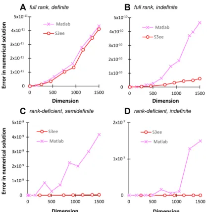
Our next aim was to compare the performance of the best variant of oscABS algorithm (S3ee) with a commercially available software able to solve complex linear systems of equations. We chose themldivide (\) algorithm of the Matlab software package from MathWorks, Inc. for that purpose. Note that Matlab’smldividealgorithm is not one specific algorithm, but consists of several algorithms, from which it chooses depending on the property of the matrixA. Themldividefunction performs several checks on the coefficient matrix to determine whether it has some special property (e.g., whether it is sparse or symmetric) and, knowing this, selects the appropriate matching solver. For example, if Ais full but not a square matrix, then it uses the QR algorithm, if not, then depending on the properties ofA, possibly the Hessenberg, Cholesky, LU, or even the LDL solver.

This means that we compared our algorithm with different solvers, selected to be most appropriate for the given problem by the Matlab program [35].

The experiments were performed with the randomly generated matrices described above.

Our results are summarized in Figure2. The S3ee algorithm outperformed Matlab algorithm in both full rank, indefinit and rank-deficient problems as well. It is clear from Figure2that the difference increases significantly as the dimension increases.

Figure 1.Comparative analysis of the four variants of the orthogonally scaled complex ABS algorithm on randomly generated dense complex systems of linear equations.

Figure 2.Comparative analysis of the S3ee implementation of the orthogonally scaled ABS algorithm and the Matlabmldividefunction on randomly generated dense complex systems of linear equations.

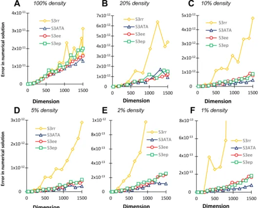
Our next set of experiments focused on the analysis of the computational accuracy of the algorithms under different matrix densities. These experiments were performed with uniformly distributed random numbers of the coefficient matrix at different densities.

As shown in Figure3, the S3ATA implementation calculated the solution most accurately and the S3rr the least accurately in most cases. The other two implementations of the orthogonally scaled complex ABS algorithms worked similar to S3ATA (i.e., within the same order of magnitude). Even at 1500 dimensions, these algorithms were able to calculate the result with an accuracy of 10⁻¹¹. It is also worth noting that reducing the density from 100% to 1% resulted in a significant improvement in computational accuracy. The accuracy increased from 10⁻¹¹to 10⁻¹³for the S3ATA, S3ee, and S3ep variants.

Figure 3.Comparative analysis of the four variants of orthogonally scaled complex ABS algorithm on randomly generated matrices with different densities.

Next, we compared the computational accuracy of our ABS-based algorithm with the Matlab algorithm on problems of different densities. As shown in Figure4, the S3ee variant of orthogonally scaled complex ABS algorithms outperformed the Matlab algorithm again.

It is worth noting that in the case of the Matlab algorithm, the change in matrix density resulted in a moderate improvement in the accuracy of the computations, as it increased from 10⁻¹¹to 10⁻¹².

In order to gain a deeper understanding of the numerical characteristics of the four variants of our algorithm, we compared the computational accuracy and execution time required to solve the 1500-dimensional systems of equations (Figure5).

Figure 4.Comparative analysis of the computational accuracy of the ABS-based S3ee algorithm and the Matlabmldivide(\) algorithm on randomly generated different-density problems.

Figure 5.Numerical properties of the four ABS-based variants and Matlab algorithm for solving 1500-dimensional random systems of equations. Panel (A) shows the computational accuracy. Panel (B) shows the execution times for our ABS-based variants in seconds. Note that the execution times of Matlab algorithms are not presented, since the Matlab built-in functions are implemented in C, which allows the algorithms to run significantly faster than our programs written in Matlab script regardless of the actual numerical performance of the algorithm.

Figure5shows that the numerical properties of the S3ee variant are the best, both in terms of computational accuracy and execution time. This may be explained by the fact that no computation is needed for parameter definitions (z_i,w_i) since the appropriate unit vectors are used and the lack of computation may also explain the accuracy since round-off errors do not accumulate. This round-off error may also explain the relatively poor numerical performance of S3ATA and S3rr.

To obtain a more comprehensive view of the numerical properties of our algorithms, we also investigated their computational accuracy for large, i.e., more than 5000 dimension problems. The dimensions of these problems were determined according to Golub and Van Loan’s suggestion [36] that for each problem, theqvalue, which is the characteristic

of the problem, remains substantially below 1. Theq=u·k_∞(A), whereu(The value of the unit round-off in Matlab is 2⁻⁵²) is unit round-off andk_∞(A)condition number of the coefficient matrix A in infinity-norm. Our results for the high-dimensional problems are summarized in Figures S1 and S2 in the Supplementary Material. Our experiments in high dimensions clearly showed that the different variants of the ABS-based algorithm solved the random problems significantly more accurately than Matlab solver. This is especially true in the rank-deficient cases, where for 5000 dimensions the Matlab function was not able to solve any problem.

3.2. Chosen Test Problems from MATLAB Gallery

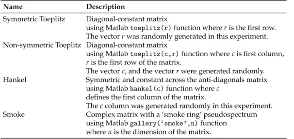
Our next experiments compared the computation accuracy of our algorithm on known complex matrices in the Matlab Gallery. Table1summarizes the problems we chose.

Table 1.Summary of test problems chosen from MATLAB Gallery.

Name Description

Symmetric Toeplitz Diagonal-constant matrix

using Matlabtoeplitz(r)function whereris the first row.

The vectorrwas randomly generated in this experiment.

Non-symmetric Toeplitz Diagonal-constant matrix

using Matlabtoeplitz(c,r)function wherecis first column, ris the first row of the matrix.

The vectorc, and the vectorrwere generated randomly.

Hankel Symmetric and constant across the anti-diagonals matrix using Matlabhankel(c)function wherec

defines the first column of the matrix.

Theccolumn was generated randomly in this experiment.

Smoke Complex matrix with a ‘smoke ring’ pseudospectrum using Matlabgallery(‘smoke’,n)function

wherenis the dimension of the matrix.

For each matrix, we tested the dimensions between 10–1500. Experiments presented in Figure6revealed that all four variants of the complex ABS algorithm were able to solve the problems with an accuracy of approximately 10⁻¹⁰and in most cases the computation error remained significantly below 10⁻¹¹. Examining the different variants of the orthogonally scaled complex ABS algorithm, we found that the S3ee and S3ep algorithms computed the problems with similar accuracy, with the S3ATA variant being the least accurate except for the Smoke problem.

Next, we compared the S3ee variant with the Matlab algorithm (see Figure7). The ABS- based algorithm slightly outperformed the Matlab algorithm on all but the Smoke matrices.

In order to gain a deeper understanding of the numerical characteristics of the four variants of our algorithm, we compared the computational accuracy and execution time required to solve the 1500-dimensional systems of equations (see Figure8).

For Matlab Gallery problems, the running properties of the algorithms are slightly different from those seen for randomly generated problems. For the first three matrix (Symmetric Toeplitz, Non-symmetric Toeplitz, Hankel) problems, we see similar results as for the randomly generated problems, the ABS-based variants giving more accurate results than the Matlab algorithm. However, for the fourth, Smoke matrix, for the first time Matlab’s algorithm gave the most accurate result tested. This fact can be partly explained by the special structure of the Smoke matrix since the diagonal of the n-dimensional Smoke matrix consists of the set of all nth roots of unity, and 1’s on its superdiagonal and 1 in the (n,1) position. It is interesting to note that the Matlab algorithm and the S3ATA variant behaved very similarly in these problems, both computing the solution with relatively large errors for the first three problems, but giving the most accurate solutions for the Smoke matrices. In the case of running speeds, it is clear that the lower computational

demand of the S3ee variant in the 1500 dimension already resulted in significantly shorter running times.

Figure 6.Comparative analysis of the four variants of the orthogonally scaled complex ABS algorithm on selected Matlab Gallery problems.

Figure 7.Comparative analysis of the computational accuracy of the ABS-based S3ee algorithm and the Matlabmldividealgorithm on selected Matlab gallery problems.

Figure 8.Numerical properties of the four ABS-based variants and the Matlab algorithm for solving 1500-dimensional Matlab Gallery problems. Panel (A) shows the computational accuracy. Panel (B) shows the execution times for our ABS-based variants in seconds.

We have also examined the behaviour of our ABS-based variants on large, i.e., more than 5000 dimensions of selected Matlab Gallery problems. Our results of the ABS-based variants are summarized in Figure S3, while the comparison of S3ee and Matlab results are summarized in Figure S4 in Supplementary Materials. For high dimensions, the numerical properties of the algorithms were very similar to those for low dimensions. Overall, of the ABS-based variants, the S3ee variant computed the most accurately and all ABS-based variants gave more accurate results than the Matlab algorithm except for the Smoke problem.

3.3. Real-Life Problems

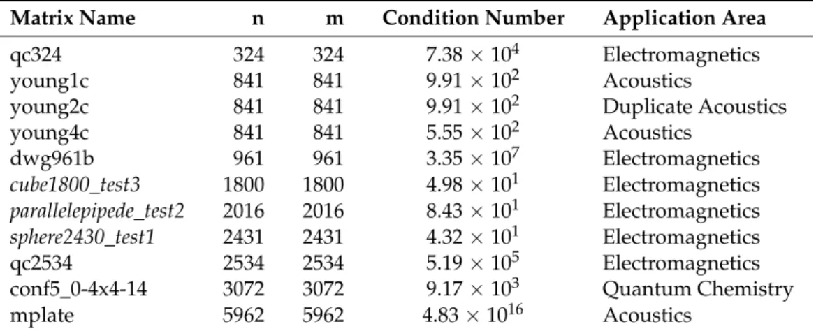
We also wanted to examine how the four variants of our ABS-based algorithm work on real-life problems. Our next experiments focused on the performance of the algorithms on examples from the SuiteSparse matrix collection [37] and from the SWUFE-Math Test Matrices Library [38]. Table2summarizes the matrices we used and their key properties.

Table 2.Summary of used real-life problems. Matrices marked by italic font come from the SWUFE- Math Test Matrices Library, while non-italicized matrices come from the SuiteSparse matrix collection.

Matrix Name n m Condition Number Application Area

qc324 324 324 7.38×10⁴ Electromagnetics

young1c 841 841 9.91×10² Acoustics

young2c 841 841 9.91×10² Duplicate Acoustics

young4c 841 841 5.55×10² Acoustics

dwg961b 961 961 3.35×10⁷ Electromagnetics

cube1800_test3 1800 1800 4.98×10¹ Electromagnetics parallelepipede_test2 2016 2016 8.43×10¹ Electromagnetics sphere2430_test1 2431 2431 4.32×10¹ Electromagnetics

qc2534 2534 2534 5.19×10⁵ Electromagnetics

conf5_0-4x4-14 3072 3072 9.17×10³ Quantum Chemistry

mplate 5962 5962 4.83×10¹⁶ Acoustics

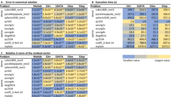
The calculation accuracies are outlined in Panel A of Figure9. It can be stated that each of the variants of the ABS-based algorithm was able to solve the problems with acceptable accuracy. For these problems, the S3rr algorithm performed best. It should be noted, however, that in most cases, the Matlab function calculated the solution most accurately.

This may partly be explained by the fact that Matlab uses different solvers for different (i.e., sparse, dense) matrices. In addition to the accuracy of the solutions and execution times, we show the relative 2-norm of the residual vectors in the PanelCto ensure that the numerical properties of our ABS-based algorithm can be compared with other published algorithms [38–40] developed to solve linear systems of equations. These comparisons revealed that our method is significantly more accurate than expected for iterative solutions.

Furthermore, some iterative methods achieved this accuracy of 10⁻⁶only after a relatively large number of iterations. In the case of the young1c problem, several algorithms needed nearly 400 steps to achieve an accuracy of 10⁻⁶[38,39], while our algorithm achieved an accuracy of 10⁻¹⁴in about twice as many steps.

Figure 9.Comparative analysis of the performance of the four variants of the orthogonally scaled complex ABS algorithm and themldivide(\) algorithm of Matlab on real-life problems. Panel (A) shows the computational accuracy. Panel (B) shows the execution times for our ABS-based variants in seconds. Panel (C) shows the relative 2-norm of the residual vector (^kb−_kbk^Axnk2

2 ).

4. Conclusions

In this paper, we presented a new ABS-based algorithm for solving complex linear systems of equations and we proved some of its basic features. We also showed a special choice of parameters of our algorithm, which ensures that the search vectors (p_i) areA^HA conjugate. A detailed numerical analysis of four variants of the ABS-based orthogonally scaled algorithm has also been provided. These variants were tested on randomly generated full and rank deficient, different-density systems of linear equations. Furthermore, the computational accuracy of the algorithm was tested on real-life problems. These numerical experiments showed that the ABS-based algorithm solved the problem with acceptable accuracy in all cases and provided more accurate results than the MATLAB built-in function in most test cases. These numerical results demonstrate the practical usefulness of the algorithm in addition to its theoretical significance.

Additionally, a valuable numerical property of our algorithm is that if we want to compute a complex system of linear equations with several right-hand sides [40], it is not necessary to recompute the matrixH_i. Instead, it is sufficient to store the vectorsp_iand recompute the updatesx_i, which can significantly reduce the computational cost. and thus our algorithm can be used effectively to solve such problems.

Supplementary Materials:The following are available online athttps://www.mdpi.com/article/10 .3390/math9192527/s1.

Author Contributions: The authors contributed equally to this work. All authors have read and agreed to the published version of the manuscript.

Funding:This research received no external funding.

Institutional Review Board Statement:Not applicable.

Informed Consent Statement:Not applicable.

Data Availability Statement:The Matlab code for the two variants of the complex ABS algorithms (S3ee, Serr) is available on GitHub, athttps://github.com/SzabinaFodor/complexABS(accessed:

2 October 2021).

Acknowledgments: The authors would like to express their sincere thanks to Attila Mócsai and the anonymous reviewers for their valuable comments and constructive suggestions that greatly improved the presentation of our work.

Conflicts of Interest:The authors declare no conflict of interest.

Abbreviations

The following abbreviations are used in this manuscript:

A^T transpose of the matrix A A the conjugate of the matrix A A^H=A^T conjugate transpose of the matrix A

References

1. Wong, S.S.M. Computational Methods in Physics and Engineering; World Scientific Publishing Co Pte Ltd.: Hackensack, NJ, USA, 1992.

2. Metzler, L.A. Taxes and subsidies in Leontief’s input-output model. Q. J. Econ.1951,65, 433–438. [CrossRef]

3. Bar-On, I.; Ryaboy, V. Fast diagonalization of large and dense complex symmetric matrices, with applications to quantum reaction dynamics. SIAM J. Sci. Comput.1997,18, 1412–1435. [CrossRef]

4. Nesemann, J.PT-Symmetric Schrödinger Operators with Unbounded Potentials; Springer: Berlin/Heidelberg, Germany, 2011.

5. Lancaster, P. Inverse spectral problems for semisimple damped vibrating systems. SIAM J. Matrix Anal. Appl.2007,29, 279–301.

[CrossRef]

6. Keller, J.B.; Givoli, D. Exact non-reflecting boundary conditions. J. Comput. Phys.1989,82, 172–192. [CrossRef]

7. Van Dijk, W.; Toyama, F. Accurate numerical solutions of the time-dependent Schrödinger equation. Phys. Rev. E2007,75, 036707.

[CrossRef]

8. Benia, Y.; Ruggieri, M.; Scapellato, A. Exact solutions for a modified Schrödinger equation. Mathematics2019,7, 908. [CrossRef]

9. Obaidat, S.; Mesloub, S. A New Explicit Four-Step Symmetric Method for Solving Schrödinger’s Equation. Mathematics2019, 7, 1124. [CrossRef]

10. Biddlecombe, C.; Heighway, E.; Simkin, J.; Trowbridge, C. Methods for eddy current computation in three dimensions. IEEE Trans. Magn.1982,18, 492–497. [CrossRef]

11. Arridge, S.R. Optical tomography in medical imaging. Inverse Probl.1999,15, R41. [CrossRef]

12. Benzi, M.; Bertaccini, D. Block preconditioning of real-valued iterative algorithms for complex linear systems. IMA J. Numer.

Anal.2008,28, 598–618. [CrossRef]

13. Day, D.; Heroux, M.A. Solving complex-valued linear systems via equivalent real formulations. SIAM J. Sci. Comput. 2001, 23, 480–498. [CrossRef]

14. Gu, X.M.; Clemens, M.; Huang, T.Z.; Li, L. The SCBiCG class of algorithms for complex symmetric linear systems with applications in several electromagnetic model problems.Comput. Phys. Commun.2015,191, 52–64. [CrossRef]

15. Wang, J.; Guo, X.P.; Zhong, H.X. Accelerated GPMHSS method for solving complex systems of linear equations. East Asian J.

Appl. Math.2017,7, 143–155. [CrossRef]

16. Li, L.; Huang, T.Z.; Ren, Z.G. A preconditioned COCG method for solving complex symmetric linear systems arising from scattering problems. J. Electromagn. Waves Appl.2008,22, 2023–2034. [CrossRef]

17. Gu, X.M.; Huang, T.Z.; Li, L.; Li, H.B.; Sogabe, T.; Clemens, M. Quasi-minimal residual variants of the COCG and COCR methods for complex symmetric linear systems in electromagnetic simulations. IEEE Trans. Microw. Theory Tech. 2014,62, 2859–2867.

[CrossRef]

18. Jacobs, D.A. A generalization of the conjugate-gradient method to solve complex systems. IMA J. Numer. Anal.1986,6, 447–452.

[CrossRef]

19. Saad, Y.Iterative Methods for Sparse Linear Systems; SIAM: Philadelphia, PA, USA, 2003.

20. Fischer, B.; Reichel, L. A stable Richardson iteration method for complex linear systems. Numer. Math. 1989,54, 225–242.

[CrossRef]

21. Bai, Z.Z.; Benzi, M.; Chen, F. Modified HSS iteration methods for a class of complex symmetric linear systems. Computing2010, 87, 93–111. [CrossRef]

22. Li, X.; Yang, A.L.; Wu, Y.J. Lopsided PMHSS iteration method for a class of complex symmetric linear systems. Numer. Algorithms 2014,66, 555–568. [CrossRef]

23. Puzyrev, V.; Koric, S.; Wilkin, S. Evaluation of parallel direct sparse linear solvers in electromagnetic geophysical problems.

Comput. Geosci.2016,89, 79–87. [CrossRef]

24. Koric, S.; Lu, Q.; Guleryuz, E. Evaluation of massively parallel linear sparse solvers on unstructured finite element meshes.

Comput. Struct.2014,141, 19–25. [CrossRef]

25. Abaffy, J.; Spedicato, E.ABS Projection Algorithms: Mathematical Techniques for Linear and Nonlinear Equations; Prentice-Hall, Inc.:

Chichester, UK, 1989.

26. Spedicato, E.; Xia, Z.; Zhang, L. ABS algorithms for linear equations and optimization. J. Comput. Appl. Math.2000,124, 155–170.

[CrossRef]

27. Fodor, S. Symmetric and non-symmetric ABS methods for solving Diophantine systems of equations. Ann. Oper. Res.2001, 103, 291–314. [CrossRef]

28. Abaffy, J.; Fodor, S. Solving Integer and Mixed Integer Linear Problems with ABS Method. Acta Polytech. Hung.2013,10, 81–98.

[CrossRef]

29. Galántai, A. Parallel ABS projection methods for linear and nonlinear systems with block arrowhead structure. Comput. Math.

Appl.1999,38, 11–17. [CrossRef]

30. Fodor, S.; Németh, Z. Numerical analysis of parallel implementation of the reorthogonalized ABS methods. Cent. Eur. J. Oper.

Res.2019,27, 437–454. [CrossRef]

31. Abaffy, J.; Fodor, S. Reorthogonalization methods in ABS classes. Acta Polytech. Hung.2015,12, 23–41.

32. Broyden, C. On the numerical stability of Huang’s and related methods. J. Optim. Theory Appl.1985,47, 401–412. [CrossRef]

33. Hegedüs, C.J. Reorthogonalization Methods Revisited. Acta Polytech. Hung.2015,12, 7–26.

34. Parlett, B. The Symmetric Eigenvalue Problem; Republished amended version of original published by Prentice-Hall; SIAM:

Philadelphia, PA, USA; Prentice-Hall: Englewood Cliffs, NJ, USA, 1980; p. 1980.

35. Attaway, D.C.Matlab: A Practical Introduction to Programming and Problem Solving; Butterworth-Heinemann Elsevier Ltd.: Oxford, UK, 2013.

36. Golub, G.H.; Van Loan, C.F.Matrix Computations, 4th ed.; Johns Hopkins University Press: Baltimore, MD, USA, 2012; Volume 3.

37. Davis, T.A.; Hu, Y. The University of Florida sparse matrix collection.ACM Trans. Math. Softw. (TOMS)2011,38, 1–25. [CrossRef]

38. Gu, X.M.; Carpentieri, B.; Huang, T.Z.; Meng, J. Block variants of the COCG and COCR methods for solving complex symmetric linear systems with multiple right-hand sides. InNumerical Mathematics and Advanced Applications ENUMATH 2015; Springer:

Berlin/Heidelberg, Germany, 2016; pp. 305–313.

39. Jing, Y.F.; Huang, T.Z.; Zhang, Y.; Li, L.; Cheng, G.H.; Ren, Z.G.; Duan, Y.; Sogabe, T.; Carpentieri, B. Lanczos-type variants of the COCR method for complex nonsymmetric linear systems. J. Comput. Phys.2009,228, 6376–6394. [CrossRef]

40. Zhong, H.X.; Gu, X.M.; Zhang, S.L. A Breakdown-Free Block COCG Method for Complex Symmetric Linear Systems with Multiple Right-Hand Sides. Symmetry2019,11, 1302. [CrossRef]