An Approach for Computing the Heat Sources in Logs Subjected to Freezing
Nencho D
ELIISKI*–Natalia T
UMBARKOVADepartment of Woodworking Machines, Faculty of Forest Industry, University of Forestry, Sofia, Bulgaria
Abstract– This study suggests an approach for computing the specific energies of the internal heat sources in logs subjected to freezing. The approach maximally considers the physics of the freezing processes of both the free and the bound water in wood. It reflects the influence on the mentioned energies of the wood density above and below the hygroscopic range. It also considers the icing degrees formed separately by both the free and bound water in the logs, as well as the influence of the fiber saturation point of each wood species on its respective amount of non-frozen water depending on temperatures below 272.15 K.
Mathematical descriptions of the specific heat energies Qv-fw and Qv-bwreleased in logs during free water freezing in the range from 0 oC to –1 oC and of the bound water below –1oC, respectively, have been executed. These descriptions are introduced in own 2D non-linear mathematical model of the freezing process of logs. For the solution of the model and computation of the energies Qv-fw and Qv-bw, a software program based on the suggested approach and mathematical descriptions was prepared in FORTRAN, which was input into the calculation environment of Visual Fortran. With the aid of the program, computations were completed to determine the energies Qv-fw and Qv-bwand their sum, Qv-totalof a beech log subjected to freezing. The beech log had a diameter of 0.24 m, a length of 0.48 m, an initial temperature of 20.5 oC, a basic density of 683 kg·m–3, and a moisture content of 0.48 kg·kg–1 during its 30 hours in a freezer at approximately –30oC.
internal heat sources / latent heat / free water / bound water / freezing / logs
Kivonat –(J\PyGV]HUDIDJ\iVQDNNLWHWWIDU|QNEHOVĘKĘPpUOHJpQHNV]iPtWiViUD. A jelen tanul- mány egy olyan módszert ír le, DPHOO\HOIDJ\iVQDN NLWHWWIDU|QN|NEHOVĘKĘIRUUiVDLQDNIDMODJRVHQHUJLiL EHFVOKHWĘN$PyGV]HUWHOMHVPpUWpNEHQILJ\HOHPEHYHV]LDV]DEDG- és kötött víztartalom fagyási folya- PDWDLQDNIL]LNDLYRQDWNR]iVDLWYDODPLQWWNU|]LDIDVĦUĦVpJpQHNKDWiViWD]HPOttett energiákra a rosttelített- ségi tartomány alatt és felett. Emellett számol a szabad- és a kötött víz által okozott jegesedés mértékével, valamint a rosttelítettségi pontnak a nem-fagyott víz mennyiségére gyakorolt hatásával 272,15 K KĘPpUVpNOHWalatt. Módszerünkkel matematikai becslést adunk a farönkökben fagyás során felszabaduló fajlagos energiákra (Qv-fw and Qv-bw) a szabad víz esetében a 0oC és –1oC közötti KĘPpUVpNOHWWDUWRPiQ\UD kötött víz esetében –1oC alatti körülményekre. A számítások eredményeit integráltuk a farönkök fagyási IRO\PDWDLW PRGHOOH]Ę VDMiW IHMOHV]WpVĦ GLPHQ]LyV QHPOLQHiULV PRGHOOQNEH $ N|]|OW PDWHPDLNDL eljárások és módszerek alapján egy FORTRAN szoftver került kifejlesztésre, mellyel a Qv-fw and Qv-bw energiák értékei számíthatók és a modell megoldható. A fejlesztett szoftvert Visual Fortran környezetbe adaptáltunk. A program segítségével egy fagyásnak kitett bükk rönk esetében kiszámoltuk a Qv-fw and Qv-bw energiákat, valamint ezek összegét, Qv-total-t$YL]VJiOWENNW|U]VPiWPpUĘMĦm hosszú volt. A kb. –30 oC-RQ YpJ]HWW IDJ\DV]WiV PHJNH]GpVH HOĘWW D U|QN NH]GHWL KĘPpUVpNOHWH o& VĦUĦVpJH kg·m–3, nedvesség tartalma pedig 0.48 kg·kg–1volt.
EHOVĘKĘIRUUiVRNOiWHQVKĘV]DEDGYtz / kötött víz / fagyás / farönk
*Corresponding author: deliiski@netbg.com; BG-1797 SOFIA, Kliment Ohridski Blvd. 10, Bulgaria
1 INTRODUCTION
The duration and energy consumption of thermally treating frozen logs in the winter to plasticize the wood for veneer production depend on the degree of icing (Chudinov 1966, 1968, Shubin 1990, Požgaj et al. 1997, Trebula – Klement 2002, Videlov 2003, Pervan 2009, Deliiski – Dzurenda 2010, Deliiski 2011, 2013b). Reports about the temperature distribution in frozen logs subjected to defrosting are limited in the accessible specialized literature (Steinhagen 1986, 1991, Steinhagen – Lee 1988, Khattabi – Steinhagen 1992, 1993, 1995, Deliiski 2004, 2009, 2011, Deliiski – Dzurenda 2010, Deliiski et al. 2015a, Hadjiski – Deliiski 2015, 2016). In addition, research into the temperature distribution in logs during the freezing process has been limited (Deliiski – Tumbarkova 2016, 2017). Thus, there is considerable scientific and practical interest in the modeling and the multi-parameter study of the freezing process of logs.
Different engineering and technological calculations require the determination of the non- stationary temperature field in logs depending on the temperature of the gaseous or liquid medium influencing them. These calculations also require information concerning the duration of logs remaining in this medium. Such calculations are completed using mathematical models that adequately describe the complex freezing processes of both the free and bound water in wood. The internal sources of latent heat of the water, which are released within the wood during water crystallization and influence the duration and energy consumption of a log’s freezing process, are an important component of these models (Deliiski – Tumbarkova 2017). No information about the approaches for quantitative determination of the internal heat sources during wood freezing exists in the available literature regarding the hydrothermal treatment of frozen wood materials.
The present paper aims to suggest an approach to compute the specific energies of internal heat sources in logs subjected to freezing; the approach takes into account, to a maximum degree, the physics of the freezing processes of both the free and bound water in wood.
Symbols:
c – specific heat capacity (J·kg–1·K–1), D – diameter (m),
L – specific latent heat (J·kg–1) or length (m), N – number of the knots of the calculation mesh, (-),
Q – internal heat source (J·m–3) or specific heat energy (Wh·m–3), R – radius (m),
r – radial coordinate: 0d r dR(m), S – shrinkage (%),
T – temperature (K): T=t+ 273.15, t – temperature (oC): t=T– 273.15, u – moisture content (kg.kg–1= %/100), z – longitudinal coordinate: 0d z dL/2 (m),
Į – heat transfer coefficients between log surfaces and the surrounding air medium (W·m–2·K–1),
O – thermal conductivity (W·m–1·K–1), U – density (kg·m–3),
ı – root square mean error (oC), IJ – time (s),
Ȍ – relative icing degree of logs or relative degree of solidification of the metal (-).
Subscripts:
avg – average (for root square mean error of calculated values of the temperature), b – basic (for wood density, based on dry mass divided to green volume), cr – crystallization,
dfr – defrosting, fr – freezing,
fsp – fiber saturation point,
ice – ice (for logs’ icing degrees or for numbers of knots of the calculation mesh),
m – medium,
M – metal,
Ms – metal in solid state, nfw – non-frozen water, 0 – initial,
p – parallel to the wood fibers, r – radial direction,
total – total (for the whole amount of knots of the calculation mesh or for energy of the latent heat sources),
v – volume,
vM – volume of the metal,
w – wood,
we – wood effective (for specific heat capacity of the wood), wL – wood with liquid water in it,
wS – wood with solid state of water (ice) in it, wUfsp – wood at fsp,
wUnfw– wood at nfw.
Superscripts:
272.15 – at 272.15 K, i.e. at –1oC, 293.15 – at 293.15 K, i.e. at 20 oC.
2 MATERIALS AND METHODS
Mathematical model of the 2D heat distribution in logs subjected to freezing
The heat conduction equation can describe the distribution mechanism in logs subjected to freezing. When log length does not exceed log diameter by more than 3 – 4 times, the heat transfer through the frontal sides of the logs cannot be neglected because it influences the temperature change of the log cross sections, which are equally distant from the frontal sides (Chudinov 1966, 1968, Shubin 1990, Deliiski 2011). In such cases, the following 2D model for the calculation of the temperature change in the longitudinal sections of the logs (i.e. along the coordinates rand z of these sections) during their freezing in an air medium can be used (Deliiski – Tumbarkova 2017):
v wp 2
2 2 wp
2 wr
2 2 wr w
we
) , , ( )
, , (
) , , ( )
, , . ( 1 ) , , ( )
, , (
z Q z r T z T
z r T
r z r T T r
z r T r r
z r T z
r c T
»¼
«¬ º ª
w W w
w O w w
W O w
»¼
«¬ º ª
w W w
w O w
»»
¼ º
««
¬ ª
w W w
w W O w
W w
W U w
(1)
with an initial condition
r,z,0 T0T (2)
and boundary conditions for convective heat transfer:
x along the radial coordinate ron the logs’ frontal surface during the freezing process:
>
( ,0, ) ( )@
) , 0 , (
) , 0 , ( d
) , 0 , ( d
fr - m wp
fr -
p W W
W O
W W D
T r
r T r r
r
T (3)
x along the longitudinal coordinate z on the logs’ cylindrical surface during the freezing:
>
(0, , ) ( )@
) , , 0 (
) , , 0 ( d
) , , 0 ( d
fr - m wr
fr -
r W W
W O
W D
W T z T
z z z
z
T . (4)
Equations (1) to (4) represent a common form of a mathematical model of 2D heat distribution in logs subjected to freezing.
Mathematical description of the internal heat sources in logs subjected to freezing
The internal heat source in logs, Qv, in eq. (1) reflects the influence of the latent heat of the water in the wood on the logs’ freezing process. As mentioned above, no information on the approaches of the quantitative determination of the heat source Qv could be found in the available literature for hydrothermal treatment of frozen wood materials. That is why, as a methodology for the determination of Qv during the freezing of logs, the present paper applies a perspective that has been applied for the determination of the internal heat source QvM during the solidification process of melted metal (Salcudean – Abdullah 1988, Dantzig 1989, Hu – Argyropoulos 1996, Mihailov – Petkov 2010). According to this methodology, the heat source QvM is equal to
W w
\ UMS crM w MS
vM L
Q . (5)
%DVHGRQWKHSK\VLFVRIWKHORJIUHH]LQJSURFHVVIRUWKHGHQVLW\RIWKHZRRGȡw, during its freezing, it could be written that
wS wL
w U U
U , (6)
wL w
wS U U
U (7)
For the numerical solution of eq. (1) it is suitable to present eq. (7) in the following form:
w wL w w
wS U
U U U
U . (8)
Using eq. (8), analogously to eq. (5), for the internal heat source in the wood it is obtained that
W w
\
w
¸¸¹
·
¨¨©
§ U
U
U W U
w
<
w
U cr-ice ice
w wL w w
ice ice cr wS
v L L
Q , (9)
where Lcr–ice is the specific latent heat of the water, also known as the “heat of crystallization”. This heat is released in the wood during the water freezing process and is
equal to
Lcr–ice= 3.34·105J·kg–1(Chudinov 1966, 1968, Efimov 1985, Pahi 2010, Deliiski – Tumbakova 2016).
Based on the data in the references cited above, the value of 3.34·105 J·kg–1 as constant for the specific latent heat for both the free and the bound water in the wood materials has been accepted in the present paper. Our wide experiments with different wood species showed
that the free water freezing occurs in the small range from 0 oC to –1 oC (Deliiski – Tumbarkova 2016). This means that the acceptance of the non-temperature dependent constant value of 3.34·105J·kg–1as a specific latent heat of the free water is correct.
We did not find data in the accessible specialized literature that reflects the temperature dependence of the specific latent heat of bound water in the wood. Rogers – Yau 1989 contains data for the specific latent heat of the sublimation and deposition from and into ice in the range from –40 oC to 0 oC (in J·g–1), which can be approximated by the following equation: Lice = 2834.2 – 0.29T – 0.004T2. Deposition is a thermodynamic process – a phase transition in which gas (or water steam) solidifies without passing through the liquid phase.
The reverse of deposition is sublimation.
Calculation of Lice with the equation given above at T = 243.15 K (i.e. at t = –30 oC, which is the lowest T reached during our experiment described below), and at T = 272.15 K (i.e. at t= –1oC) show that the obtained results differ from each other by only 2.7%. Because liquid water is a far more stable substance compared to steam, it can be surmised that the specific latent heat of the bound water at t= –30 oC differs negligibly from its value at t= –1oC.
This allowed us to accept a constant value of the specific latent heat of the bound water during log freezing equal to 3.34·105J·kg–1.
Designating the expression in the brackets from eq. (9) with K\, i.e.
w wL w
U U
\ U
K (10)
and substituting eq. (10) into eq. (9), the following final expression for Qvis obtained:
W w
\
w U
\ ice ice - cr w
v K L
Q . (11)
Mathematical description of the internal heat source in logs during freezing of the free water According to eq. (11), during the free water freezing process in wood, the consequent formed source of latent heat Qv-fwis equal to
W w
\
w U
\ ice-fw ice
- cr w fw fw
-
v K L
Q , (12)
where based on the physics of the process and on the form of eq. (10), it is obtained that
w wUfsp w
fw U
U U
K\ , (13)
given that <ice-fw is the relative icing degree of the logs, which results from the freezing of the free water in them. An approach and an algorithm for its calculation are given in Deliiski – Tumbarkova (2017).
The difference Uw – UwUfsp in the right-hand part of eq. (13) reflects the entire mass of free water (in kg), which is contained in 1 m3of the logs.
7KHZRRGGHQVLWLHVȡwandUwUfsp, which participate in eq. (13), are determined above the hygroscopic range according to the below equations (Chudinov 1968, Pervan 2009, Deliiski 'HOLLVNLHWDOE+UþND
) 1
b (
w U u
U , (14)
) 1 ( fsp
b wUfsp U u
U . (15)
Mathematical description of the internal heat source in logs during bound water freezing Analogously to eq. (11) and eq. (12), during the freezing of the bound water in the wood, the consequently formed source of latent heat in it,Qv-bw, is equal to
W w
\
w U
\ ice-bw ice
- cr w bw bw
-
v K L
Q , (16)
where based on the physics of the process and on the form of eq. (10), it is obtained that
w wUnfw wUfsp
bw U
U U
K\ , (17)
given that <ice-bw is the relative icing degree of the logs, which results from the freezing of the bound water in them. An approach and an algorithm for its calculation are given in Deliiski – Tumbarkova (2017);
UwUnfw – density of the wood, determined according to the following equation in relation to the present entirely liquid quantity of water in the wood (kg·m–3), corresponding to the current temperature Ɍ< 272.15 K (Chudinov 1966, Deliiski 2013b):
fsp272.15 nfwv b nfw wUnfw
1 100 1
u S u
u
U
U , (18)
272.15
ufsp – fiber saturation point of the wood (kg·kg–1) at Ɍ = 272 K (i.e. at t = –1 oC).
At this temperature the freezing of the bound water begins in the wood.
While observing the freezing of the logs from various wood species with different moisture contents above the hygroscopic range during our wide experiments, we determined that freezing of the bound water begins at t= –1oC (Deliiski – Tumbarkova 2016) and not at t= –2 oC, which was determined by Chudinov (1966, 1968) and, consequently, was widely accepted in the relevant literature.
The fiber saturation point ufsp272.15 can be calculated according to the following equation (Stamm 1964, Deliiski 2013a):
021 .
293.15 0
fsp 272.15
fsp u
u , (19)
where 293.15
ufsp is the standardized value of the fiber saturation point of the wood (kg·kg–1) at 293.15 K, i.e. at 20 ɨɋ
unfw– non-frozen quantity of bound water in the wood (kg·kg–1) at a given temperature Ɍ< 272.15 K. It can be calculated according to the equation (Chudinov 1968, Deliiski 2013b):
0.12exp>
0.0567272.15
@
@ 213.15 K 272.15 K12 .
0 fsp272.15
nfw u T dTd
u . (20)
Experimental research of the log freezing process
Experimentally obtained data about the change in the temperature field in logs during their freezing were required for the application and verification of the approach suggested above.
Consequently, we carried out such experiments.
The logs subjected to experimental research, produced from the sapwood of freshly felled beech trunks (Fagus sylvaticaL.), had diameters of D= 240 mm, lengths of L= 480 mm, and moisture contents above the hygroscopic range.
Before the experiments, four holes, with differing lengths and diameters of 6 mm were drilled into each log. Sensors with long metal casings were positioned in these four holes to measure wood temperature during the experiments. The point coordinates of the logs are as follows:
Point 1: along the radius r=30 mm and along the length z=120 mm;
Point 2: along the radius r =60 mm and along the length z =120 mm;
Point 3: along the radius r =90 mm and along the length z =180 mm;
Point 4: along the radius r=120 mm and along the length z=240 mm.
These characteristic point coordinates make it possible to sense the impact of the heat fluxes simultaneously in radial and longitudinal directions on the temperature distribution in logs during the freezing process.
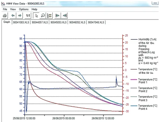
For log freezing according to the methodology suggested by the authors (Deliiski – Tumbarkova 2016), a horizontal freezer with a fitted with temperature sensors and was horizontally situated on a special stand in the open freezer that was initially at room temperature. The freezer was then closed and switched on to full power; the temperature of the freezing air medium in the freezer, tm, was lowered gradually until it reached approximately –30oC (Figure 1).
The automatic measuring and recording of the temperature and humidity of the air processing medium in the freezer and the temperature in the 4 points in the logs during the experiments was implemented with the help of Data Logger type HygroLog NT3 produced by the Swiss firm ROTRONIC AG (http:/www.rotronic.com).
As an example, Figure 1 presents the change in the temperature of the processing air medium, tm DQGLQLWVKXPLGLW\ijm, and also in the temperature in four characteristic points of a beech log with u= 0.48 kg·kg–1DQGȡb = 683 kg·m–3 during 30 h of freezing. The record of all data was made automatically by Data Logger in 5 minute intervals.
Figure 1. Experimentally determined change in tmijm, and t in 4 characteristic points of beech log with D = 0.24 m, L = 0.48 m, u = 0.48 kg·kg–1ȡb = 683 kg·m–3
(i.e.ȡw = 1010.8 kg·m–3), and t0 = 20.5 oC during its 30 h freezing
3 RESULTS AND DISCUSSION
The mathematical descriptions of the internal heat sources Qv-fw and Qv-bw created above and the mathematical descriptions of the thermo-physical characteristics of frozen and non-frozen wood suggested earlier (Deliiski 2004, 2009, 2011, 2013a) are introduced in the mathematical model of the log freezing process, which consists of eqs. (1) – (20). This model has been solved with the help of explicit schemes of the finite difference method, analogous to the one used and described in (Deliiski 1977, 1988, 2009, 2011, Deliiski et al. 2015a) for the solution of a model of the heating process of prismatic and cylindrical wood materials. For this purpose, the calculation mesh has been built on ¼ of the longitudinal section of the log due to the circumstance that this ¼ is mirror symmetrical towards the remaining ¾ of the same section (Figure 2).
Computation of 2D non-stationary temperature distribution in logs during their freezing For the numerical solution of the mathematical model, a software program was prepared in FORTRAN in the calculation environment of Visual Fortran Professional. With the help of the program, computations were made for the determination of the 2D non-stationary change of t in ¼ of the longitudinal section of the beech log whose experimentally determined temperature distribution is shown on Figure 1as an example.
7KHPRGHOZDVVROYHGZLWKVWHSǻr ǻz= 6 mm along the coordinates r and zand with the same initial and boundary conditions, as they were during the experimental research. This means that the calculation mesh consists of 20 x 40 = 800 knots: 20 alongr and 40 along z.
The solution of the model gives the non-stationary change of the temperature in calculation mesh knots (Figure 2) and of different energy characteristics of logs subjected to freezing.
Figure 2. Positioning of the knots of the calculation mesh on ¼ of the longitudinal section of a log subjected to freezing
During the solving of the model, the mathematical descriptions of the thermo-physical characteristics of beech wood with fiber saturation point 293.15 1
fsp 0.31 kgkg
u and volume
shrinkage Sv = 17.3% were used (Nikolov – Videlov 1987).
The curvilinear change shown in Figure 1 in the freezing air medium temperature, Ɍmfr, with high accuracy (correlation 0.99 and Root Square Mean Error (RSME) 0.14 oC) has been approximated with the help of the software package Table Curve 2D (http://www.sigmaplot.co.uk/products/tablecurve2d/tablecurve2d.php) by the equation
fr 2 5 . fr 1 5 fr
. fr 0
5 . fr 1 5 fr
. fr 0 fr fr
m 1 W W W W
W W W
b d f h ɟ g
c
Ɍ a , (21)
whose coefficients are equal to:
ɚfr = 293.0642230, bfr = –0.01985592, cfr= –5.66878889, dfr = –0.000298843, efr = 0.080801194, ffr = –6.7184·10–7, gfr = –0.00019564, and hfr = –1.7404·10–10. Equation (21) was used for the solving of eqs. (3) and (4) of the model.
Figure 3 presents the change in tm-fr , log surface temperature ts, and t of 4 points of the studied beech log, which have the same coordinates, as during the experimental research.
The comparisons of the analogical curves in Figure 1 and Figure 3show good qualitative and quantitative conformity between the calculated and experimentally determined changes in the complicated temperature field of the log during its freezing. It was calculated that the RSMEIRUDOOVWXGLHGIRXUSRLQWVLQWKHORJLVıavg = 1.42 oC.
Figure 3. Calculated with the model change in tm-fr , ts, and t of 4 characteristic points of the studied beech log during its 30 h freezing
&KDQJHRIORJLFLQJGHJUHHVȌice-fw DQGȌice-bw
A logical condition in the software for the model’s solution that registers and records the moments when the temperature of each knot decreases below 273.15 K (i.e. below 0 oC) and then registers and records temperature conditions for the crystallization of the free water separately for each knot has been introduced earlier (Deliiski – Tumbarkova 2016).
This means that the current number of the knots in which the free water already
“crystallizes”, Nice-fw, has been constantly determined synchronously with the obtaining of the temperature distribution. The relationship between Nice-fw and the total number of knots of the entire calculation mesh, Nice-total = 800, is used for the estimation of the current relative icing GHJUHHRIORJVȌice-fw, which has happened by the freezing of the free water up to the present moment of log’s cooling.
The relative icing degree of logs, which is caused by the freezing of the bound water in WKHPȌice-bw, has been estimated according to a similar but more complicated approach given in (Deliiski – Tumbarkova 2017). A logical condition to solve the model in the software has also been introduced. This condition registers and records the moments when the temperature of each of the knots decreases below 272.15 K (i.e. below –1 oC) and then temperature conditions for the crystallization of the bound water separately for each knot arise.
Figure 4SUHVHQWVWKHFDOFXODWHGFKDQJHRIORJLFLQJGHJUHHVȌice-fwDQGȌice-bw during the 30 h freezing process of the studied beech log (Deliiski – Tumbarkova 2017).
)LJXUH&KDQJHLQȌice-fwDQGȌice-bw during the freezing of the studied beech log 7KHLFLQJGHJUHHȌice-fwvaries from 0 to 1 (Figure 4). It has a value of 0 during the first 2.92 hours the log spends in the freezer when all the water in the wood is in a liquid state.
This icing degree becomes equal to 1 after 14.08 h when the free water has frozen completely.
7KHLFLQJGHJUHHȌice-bw varies from 0 to 0.486 (Figure 4). It has a value of 0 during the first 3.50 hours the log spends in the freezer, while the temperature of the peripheral layers of the log decreases below –1 oC and the freezing of the bound water in these layers starts. This icing degree becomes equal to 0.486 at the end of the 30 h in the freezer. The calculated average log mass temperature is then equal to –26.38 oC (i.e. 246.77 K) and the calculated according to eq. (21) amount of the non-frozen water unfw is equal to 0.170 kg·kg–1. This value of unfw and the value ufsp272.15 0.310.021 0.331 kgkg1 (see eq. (20)) ensure a YDOXHRIȌice-bw= 0.486 (see equation
272.15 fsp bw nfw
ice 1
u u
< given in Deliiski – Tumbarkova (2017)). This means that 1 – 0.486 = 0.514 relative parts (i.e. 51.4%) of the bound water in the studied beech log remains in a liquid state at the end of 30 h of freezing when the calculated according to eq. (22) temperature in the freezer becomes equal to tm-fr= –29.69oC (Figure 3) and the average log mass temperature is equal to –26.38oC.
Change of the specific energies of the internal heat sources Qv-fw and Qv-bw
Figure 5 presents the calculated change of specific energies of the internal heat sources Qv-fw and Qv-bw, and their sum Qv-total = Qv-fw + Qv-bw during the 30 h freezing process of the studied beech log. The values of the heat sources are calculated as specific (for 1 m3 wood) heat energies in Wh·m–3instead of in J·m–3. For this purpose, the values obtained by eqs. (12) and (16) have been divided by 3600.
During the first 17.00 h of the freezing process, the energies Qv-fw and Qv-total increase according to three mutually connected almost linear sections. During the first 2.92 h, when the entire amount of the free and bound water in the log is in a liquid state, these energies remain equal to 0. After that they increase rapidly until reaching 52.27 Wh·m–3 and 65.34 Wh·m–3 respectively at the end of the freezing of the free water in the log, which takes 14.08 h. From the 14.08th h to 17.00thh, the energy Qv-fw remains constant and equal to 52.27Wh·m–3 and the energy Qv-total increases from 65.34 Wh·m–3 to 70.25 Wh·m–3.
Figure 5. Change in Qv-fw, Qv-bw, and Qv-total during the freezing of the studied beech log During the first 3.50 h, when all the bound water in the log is in a liquid state, the energy Qv-bw remains equal to 0. From 3.50th h to 17.00th h, when the gradual crystallization of the bound water in all knots of the calculation mesh (incl. in the log center) has begun, the specific energy Qv-bw increases exponentially from 0 to 17.98 Wh·m–3.
After the 17.00th h, the energy Qv-fw is equal to 0 (all the free water is frozen) and the energy Qv-bwdecreases exponentially; at the end of 30 h of freezing process, it reaches a value of 7.31 Wh·m–3. From the 17.00th h to 30.00th h of the freezing process, the total energy Qv-
total is equal to Qv-bw. The reason for the decreasing of Qv-bw during this time interval is the decrease of the first derivative of the icing degree <ice-bwin eq. (16) due to the decreasing slope of the dependence of this icing degree on the time during this interval in comparison to its slope prior to that (Figure 4).
We executed extensive simulations to verify the mathematical model given above and to study the freezing process of logs from various wood species with different moisture contents.
By varying the values of the energies Qv-fw and Qv-bwwe determined that:
x the larger values of Qv-fw in comparison to those calculated by eq. (12) cause an acceleration of the computed freezing process, i.e. they cause a shortening of the horizontal sections of the temperatures in the log’s central layers in the range between 0 oC and –1oC (Figure 1 and Figure 3). On the contrary, the lower values of Qv-fw in comparison to those calculated by eq. (12) cause a deceleration of the computed freezing process of the logs;
x the larger values of Qv-bw in comparison to those calculated by eq. (16) make the curves of the temperature field of the log below –1 oC steeper. On the contrary, the lower values of Qv-fw in comparison to those calculated by eq. (16) make the mentioned curves more lenient.
During our simulations with the model, using the approach suggested above and the mathematical descriptions of Qv-fw and Qv-bw, we obtained good qualitative and quantitative conformity between the calculated and experimentally determined temperature distribution in the log’s longitudinal section during the whole process of the freezing of both the free and the bound water not only in the studied beech log for the purposes of this paper, but also many other logs above the hygroscopic range (including the poplar logs presented in Deliiski – Tumbarkova (2016, 2017)).
The heat energies for the freezing of the free and bound water are not equal to the specific latent heat of the water. As pointed out in (Deliiski – Tumbarkova 2016), the latent heat is used for description of the thermal energy only, which is needed for the change of the aggregate state of a given substance without changing its temperature.
In (Chudinov 1966, 1968, Deliiski 2004, 2011, 2013b), it has been shown that the energies required for the freezing of the free and bound water (or for the melting of the ice formed by them) in the wood depend mainly on the specific heat capacity of the free water in a frozen state, cfw, and on the specific heat capacity of the bound water in a frozen state, cbw, respectively. Both specific heat capacities depend on the specific latent heat of the water.
In addition, cfw depends on the amount of free water in the wood and does not depend on the temperature because the free water freezes in the small range from 0 oC to –1oC.
The specific heat capacity cbw depends on the wood moisture content and on the temperature since the bound water freezes gradually in the range from –1 oC to the set or desired end temperature of the freezing, Ɍend (Deliiski 2013b, 2013c). However, even at the lowest climate temperatures on the earth about 0.12 kg·kg–1 of the bound water remains in a non-frozen state (Chudinov 1968).
4 CONCLUSIONS
The present paper describes an approach offered by the authors for the computation of the specific energies of the internal heat sources in logs subjected to freezing.
This approach takes into account, to a maximum degree, the physics of the freezing process of both the free and the bound water in the wood. It reflects the influence of the latent heat of the water in the wood on these energies. It also considers the wood density above and below the hygroscopic range, the icing degrees of the logs formed separately by both the free and bound water at each moment of log freezing, and the influence of the fiber saturation point of each wood species on its non-frozen water depending on the current temperature in the logs below 272.15 K.
Mathematical descriptions of the specific heat energies Qv-fw and Qv-bw, released in logs during the freezing of the free water in the range from 0 oC to –1 oC, and of the bound water below –1 oC, respectively, have been carried out. These descriptions are introduced in our own 2D non-linear mathematical model of the freezing process of logs.
A software program for the solution of the model and computation of the energies Qv-fw
and Qv-bw according to the suggested approach and mathematical descriptions has been prepared in FORTRAN, which has been input in the calculation environment of Visual Fortran Professional developed by Microsoft.
With the help of the program, computations for the determination of the energies Qv-fw and Qv-bw and their sum, Qv-total, have been completed as an example for the case of a beech log with a diameter of 0.24 m, length of 0.48 m, initial temperature of 20.5 oC, basic density of 683 kg·m–3, and moisture content of 0.48 kg·kg–1subjected to 30 h of freezing in a freezer at about –30oC.
It has been determined that the values of the specific heat energies Qv-fw, Qv-bw, and Qv- totalof the studied log change according to complex relationships, as follows:
x the energy Qv-fw, which is released by the freezing of only the free water in the wood, changes from 0 to 52.27 Wh·m–3 during the time from 2.92nd h to 14.08th h of the freezing process;
x the energy Qv-bw, which is released by the freezing of a portion of the bound water in the wood, changes from 0 to 17.98 Wh·m–3 during the time from 3.50th h to 17.00th h of the freezing process. After the 17.00th h this energy decreases exponentially and at the end of 30 h of freezing process it reaches a value of 7.31 Wh·m–3;
x the total energy Qv-total = Qv-fw + Qv-bw changes from 0 to 70.25 Wh·m–3 during the time from 2.92ndh to 17.00th h of the freezing process. From the 17.00thh to 30.00th h the energy Qv-total is equal to Qv-bw.
By applying the suggested approach for the computation of Qv-fw and Qv-bw during our simulations with the mathematical model, we observed good conformity between the calculated and experimentally determined changes in the temperature field during the freezing of logs from different wood species with different moisture contents.
The overall RSME for the studied four characteristic points in the logs does not exceed 5% of the temperature ranges between the initial and the end temperatures of the logs subjected to freezing. This proves the suitable adequacy of the model as well as the correctness of the suggested approach.
The validation of the model with curvilinear change in the temperature of the freezing air medium will allow us, in the future, to solve the model (mutually connected with other our model of the logs’ defrosting process) with curvilinear changing of the climate temperature (Deliiski 1988) over many winter days and nights. It will also allow for scientific calculations based the temperature distribution, icing degrees, and different energy characteristics of logs for each desired moment.
The approach for the computation of the specific energies of the internal heat sources in logs subjected to freezing suggested in this paper could be further applied in the development of analogous models; for example, for the calculation of the temperature fields and the energy consumption during the freezing of different wooden and other capillary-porous materials.
Acknowledgements: This document was supported by the grant No BG05M2OP001-2.009- 0034-C01 “Support for the Development of Scientific Capacity in the University of Forestry”, financed by the Science and Education for Smart Growth Operational Program (2014-2020) and co-financed by the EU through the European structural and investment funds.
REFERENCES
CHUDINOV, B.S. (1966): Teoreticheskie issledovania teplofizicheskih svoystv i teplovoy obrabotki dreveciny [Theoretical Research of Thermo-physical Properties and Thermal Treatment of Wood]. Dissertation for DSc., SibLTI, Krasnoyarsk, USSR (in Russian)
CHUDINOV, B.S. (1968): Teoria teplovoy obrabotki drevesiny [Theory of Thermal Treatment of Wood]. Nauka, Moscow, USSR, 255 p. (in Russian)
DANTZIG, J. (1989): Modelling Liquid-solid Phase Changes with Melt Convection. International Journal for Numerical Methods in Engineering 28 (8): 1769–1785.
https://doi.org/10.1002/nme.1620280805
DELIISKI, N. (1977): Berechnung der instationären Temperaturverteilung im Holz bei der Erwärmung durch Wärmeleitung. Teil 1: Mathematisches Modell für die Erwärmung des Holzes durch Wärmeleitung [Calculating the unsteady-state distribution of temperature during conductive heating of wood. Part 1: Mathematic model conductive heatingof wood]. Holz Roh- und :HUNVWRIIí(in German)
DELIISKI, N. (1988): Thermische Frequenzkennlinien von wetterbeanspruchten Holzbalken [Thermal frequency characteristics of weathered wooden beams]. Holz als Roh- und Werkstoff 20 (2): 59–
65. (in German)https://doi.org/10.1007/BF02612530
DELIISKI, N. (2004): Modelling and Automatic Control of Heat Energy Consumption Required for Thermal Treatment of Logs. Drvna Industrija 55 (4): 181–199.
DELIISKI, N. (2009): Computation of the 2-dimensional Transient Temperature Distribution and Heat Energy Consumption of Frozen and Non-IUR]HQ/RJV:RRG5HVHDUFKí
DELIISKI, N. (2011): Transient Heat Conduction in Capillary Porous Bodies. In Ahsan A. (ed) Convection and Conduction Heat Transfer. InTech Publishing House, Rieka: 149–176.
https://doi.org/10.5772/21424
DELIISKI, N. (2013a): Computation of the Wood Thermal Conductivity during Defrosting of the Wood. Wood research 58 (4): 637–650.
DELIISKI, N. (2013b): Modelling of the Energy Needed for Heating of Capillary Porous Bodies in Frozen and Non-frozen States. Lambert Academic Publishing, Scholars’ Press, Saarbruecken, Germany, 116 p.
DELIISKI, N. (2013c):Modelling of the Energy Needed for Melting of the Ice in Frozen Wood above the Hygroscopic Diapason. Wood Design and Technology, Vol.2, No.1, p.42–52, Ss.Cyril and Methodius University – Skopje.
DELIISKI, N. – DZURENDA, L. (2010): Modelling of the Thermal Processes in the Technologies for Wood Thermal Treatment. TU Zvolen, Slovakia, 224 p. (in Russian)
DELIISKI, N. – BREZIN, V. – TUMBARKOVA, N. (2015a): Modelling of the 1D Convective Heat Exchange Between Logs Subjected to Freezing and to Subsequent Defrosting and the Surrounding Environment. Acta Silvatica et Lignaria Hungarica 11 (1): 77–
88.https://doi.org/10.1515/aslh-2015-0006
DELIISKI, N. – DZURENDA, L. – TUMBARKOVA, N. – ANGELSKI, D. (2015b): Computation of the Temperature Conductivity of Frozen Wood during its Defrosting. Drvna Industrija 66 (2): 87–96.
https://doi.org/10.5552/drind.2015.1351
DELIISKI, N. – TUMBARKOVA, N. (2016): A Methodology for Experimental Research of the Freezing Process of Logs. Acta Silvatica et Lignaria Hungarica 12 (2): 145–156.
https://doi.org/10.1515/aslh-2016-0013
DELIISKI, N. – TUMBARKOVA, N. (2017): An Approach and an Algorithm for Computation of the Unsteady Icing Degrees of Logs Subjected to Freezing. Acta Facultatis Xilologiae Zvolen 59 (2):
91–104.
EFIMOV, S.N. (1985): Temperaturnaya zavisimost tepla kristallizacii vody [Temperature Dependence of the Heat of Water Crystallization]. Engineering-Physical Journal of the Institute of Physic- Technical Problems of the Nord, Siberian Department of the Academy of Sciences of USSR, Yakutsk, 49(4): 658–664. (in Russian)
HADJISKI, M. – DELIISKI, N. (2015): Cost Oriented Suboptimal Control of the Thermal Treatment of Wood Materials. IFAC-PapersOnLine 4824 (2015): 54–59.
https://doi.org/10.1016/j.ifacol.2015.12.056
HADJISKI, M. – DELIISKI, N. (2016): Advanced Control of the Wood Thermal Treatment Processing.
Cybernetics and Information Technologies, Bulgarian Academy of Sciences 16 (2): 179197.
https://doi.org/10.1515/cait-2016-0029
H5ý.$, R. (2017): Model in Free Water in Wood. Wood Research 62 (6): 831–837.
HU, H. – ARGYROPOULOS, S. (1996): Mathematical Modelling of Solidification and Melting: A Review. Modelling and Simulation in Materials Science and Engineering 4: 371–396.
https://doi.org/10.1088/0965-0393/4/4/004
KHATTABI, A. – STEINHAGEN, H.P. (1992): Numerical Solution to Two-dimensional Heating of Logs.
Holz als Roh- und Werkstoff 50 (7-8): 308–312.https://doi.org/10.1007/BF02615359
KHATTABI, A. – STEINHAGEN, H.P. (1993): Analysis of Transient Non-linear Heat Conduction in Wood Using Finite-difference Solutions. Holz als Roh- und Werkstoff 51 (4): 272–278.
https://doi.org/10.1007/BF02629373
KHATTABI, A. – STEINHAGEN, H.P. (1995): Update of “Numerical Solution to Two-dimensional Heating of Logs”. Holz als Roh- und Werkstoff 53(2): 93–94.https://doi.org/10.1007/BF02716399
MIHAILOV, E. – PETKOV, V. (2010): Cooling Parameters and Heat Quantity of the Metal During Continuous Casting of Blooms. International Review of Mechanical Engineering 4 (2): 176–184.
NIKOLOV, S. – VIDELOV, CH. (1987): Manual for Wood Drying. Zemizdat, Sofia, 394 pp.
PAHI, S. (2010): Understanding specific latent heat. Lesson 4.3 – Understanding thermal latent heat.
Bidang Sains dan Matematik
PERVAN, S. (2009): Technology for Treatment of Wood with Water Steam. University in Zagreb (in Croatian)
POŽGAJ, A. – CHOVANEC, D. – KURJATKO, S. – BABIAK, M. (1997): Štruktúra a vlastnosti dreva [Structure and Properties of Wood]. 2ndedition, Priroda a.s., Bratislava, 485 p. (in Slovakian) ROGERS, R.R. – YAU, M. K. (1989): A short Course in Cloud Physics (3rded.). Pergamon Press, ISBN
0-7506-3215-1.
SALCUDEAN, M. – ABDULLAH, Z. (1988): On the Numerical Modelling of Heat Transfer during Solidification Processes. International Journal for Numerical Methods in Engineering 25: 445–473.
https://doi.org/10.1002/nme.1620250212
SHUBIN, G.S. (1990): Sushka i teplovaya obrabotka drevesiny [Drying and Thermal Treatment of Wood]. Lesnaya Promyshlennost, Moskow, URSS, 337 p. (in Russian)
STAMM, A. J. (1964): Wood and Cellulose Science. Ronald Press, New York.
STEINHAGEN, H.P. (1986): Computerized Finite-difference Method to Calculate Transient Heat Conduction with Thawing. Wood Fiber Science 18 (3): 460–467.
STEINHAGEN, H.P. (1991): Heat Transfer Computation for a Long, Frozen Log Heated in Agitated Water or Steam – A Practical Recipe. Holz als Roh- und Werkstoff 49 (7-8): 287–290.
https://doi.org/10.1007/BF02663790
STEINHAGEN, H.P. – LEE, H.W. (1988): Enthalpy Method to Compute Radial Heating and Thawing of Logs. Wood Fiber Science 20 (4): 415–421.
TREBULA, P. – KLEMENT, I. (2002): Drying and Hydro-thermal Treatment of Wood. Technical University in Zvolen, Slovakia, 449 p. (in Slovakian)
VIDELOV, CH. (2003): Sushene i toplinno obrabotvane na darvesinata [Drying and Thermal Treatment of Wood]. University of Forestry in Sofia, Sofia, 335 p. (in Bulgarian)