Efficiently sampling the realizations of bounded, irregular degree sequences of bipartite and directed graphs
Pe´ter L. Erdős☯¤*, Tama´s Ro´ bert Mezei☯, Istva´n Miklo´ s☯, Da´niel Solte´sz☯ Alfre´d Re´nyi Institute of Mathematics, Hungarian Academy of Sciences, Budapest, Hungary
☯These authors contributed equally to this work.
¤ Current address: Rea´ltanoda u 13-15, Budapest, H-1053, Hungary
*erdos.peter@renyi.mta.hu
Abstract
Since 1997 a considerable effort has been spent on the study of the swap (switch) Markov chains on graphic degree sequences. All of these results assume some kind of regularity in the corresponding degree sequences. Recently, Greenhill and Sfragara published a breakthrough paper about irregular normal and directed degree sequences for which rapid mixing of the swap Markov chain is proved. In this paper we present two groups of results. An example from the first group is the following theorem: let~dbe a directed degree sequence on n vertices. Denote byΔthe maximum value among all in- and out-degrees and denote byj~Ejthe number of edges in the realization. Assume furthermore that
D< 1ffiffi
p2
ffiffiffiffiffiffiffiffiffiffiffiffiffiffiffi j~Ej 4 q
. Then the swap Markov chain on the realizations of~dis rapidly mixing. This result is a slight improvement on one of the results of Greenhill and Sfragara. An example from the second group is the following: let d be a bipartite degree sequence on the vertex set U]V, and let 0<c1c2<|U| and 0<d1d2<|V| be integers, where c1d(v)c2: 8v2V and d1d(u)d2:8u2U. Furthermore assume that (c2−c1−1)(d2−d1−1)<max {c1(|V|−d2), d1(|U|−c2)}. Then the swap Markov chain on the realizations of d is rapidly mix- ing. A straightforward application of this latter result shows that when a random bipartite or directed graph is generated under the Erdős—Re´nyi G(n, p) model with mild assumptions on n and p then the degree sequence of the generated graph has, with high probability, a rapidly mixing swap Markov chain on its realizations.
Introduction
An important problem in network science is to algorithmically construct typical instances of networks with predefined properties, often expressed as graph measures. In particular, special attention has been devoted to sampling simple graphs (in our paper only graphs without paral- lel edges and loops are considered) with a given degree sequence. In 1997 Kannan, Tetali, and Vempala ([1]) proposed the use of the so-called switch Markov chain approach, which had already been used in statistics. We call this the swap Markov chain approach.
a1111111111 a1111111111 a1111111111 a1111111111 a1111111111
OPEN ACCESS
Citation: Erdős PL, Mezei TR, Miklo´s I, Solte´sz D (2018) Efficiently sampling the realizations of bounded, irregular degree sequences of bipartite and directed graphs. PLoS ONE 13(8): e0201995.
https://doi.org/10.1371/journal.pone.0201995 Editor: Arndt von Haeseler, Max F Perutz Laboratories GmbH, AUSTRIA
Received: May 16, 2018 Accepted: July 25, 2018 Published: August 13, 2018
Copyright:©2018 Erdo˝s et al. This is an open access article distributed under the terms of the Creative Commons Attribution License, which permits unrestricted use, distribution, and reproduction in any medium, provided the original author and source are credited.
Data Availability Statement: All relevant data are within the paper.
Funding: The authors of this paper were supported in part by the National Research, Development and Innovation Office | NK- FIH grant K 116769 and KH 126853. IM was supported in part by the National Research, Development and Innovation Office | NKFIH grant SNN 116095. DS was supported in part by the National Research, Development and Innovation Office | NKFIH grants K 108947 and K 120706. The WEB page of the founder is:https://
www.nkh.gov.hu/en/web/english/. The funders had
The swap operation exchanges two disjoint edgesacandbdin the realizationGwithad andbcif the resulting configurationG0is again a simple graph (we denote this operation byac, bd)ad,bc). (For details see the next section). It is a well-known fact that the set of all possible realizations of a graphic degree sequence is connected under this operation. (See, for example, Petersen [2] or Havel [3] and Hakimi [4]). An analogous result applies for the swap operation defined on bipartite graphs. (See, for example, Gale [5]). Here we have to be careful, as not every edge exchange is eligible: on a bipartite graph we must ensure that verticesaandd belong to different vertex classes.
In the literature, the name switch operation is also used, however, in our approach this lat- ter is an operation on integer matrices slightly generalizing the swap operation. (See the sec- tions on the analysis of the swap sequences).
The situation is more complicated in case of directed degree sequences. In this case for every vertex the number of incoming edges (in-degree) and the number of outgoing edges (out-degree) is given in the degree bi-sequence. Here theac,bd)ad,bctype exchange pre- serves the degree bi-sequence if both before and after the swap operationaandbare tails of the directed edges. However, imagine that our graph~Gis a directed triangleC3
!whileH~is the oppositely directedC3
. Both graphs have the same degree bi-sequence d = ((1, 1, 1); (1, 1, 1)). It is clear that there is only one way to transform the first one into the second one: if we exchange three edges and three non-edges in~G. We will call this operation a triple swap and the previously defined “classical” one as a double swap. Kleitman and Wang proved in 1973 ([6]) that any two realizations of a given graphic degree bi-sequence can be transformed into each other using these two operations. The same fact was re-discovered in 2010 (see [7]).
The swap Markov chains corresponding to the most common graph models are irreducible, aperiodic, reversible (obey detailed balance), have symmetric transition matrices, and thus have uniform global stationary distributions.
In their paper [1], Kannan, Tetali and Vempala conjectured that all these Markov chains are rapidly mixing. The first rigorous proof in this topic is due to Cooper, Dyer and Greenhill for regular graphs ([8]). Now, twenty years after the KTV conjecture, we are still far, probably very far, from proving it in its full generality. However, many partial results have been proved;
those which play some role in this paper are summarized in the following theorem:
Theorem 1.The swap Markov chain mixes rapidly for the following degree sequences:
(A). dis a regular directed degree sequence.
(B). dis ahalf-regularbipartite degree sequence.
(C). dbelongs to analmost-half-regularbipartite graph.
(D). dis an almost-half-regular bipartite degree sequence, where every realization must avoid a fixed (partial) matching.
(E). dis a directed degree sequence with2dmax 14 ffiffiffiffiffi pM
,where M is the sum of the in- degrees (or out-degrees), and where the set of all realizations under study is irreducible under the double swap operation.
There exist similar results on (normal) degree sequences as well, but their proofs are not fully “compatible” with the proof of the above results (except case D). To our knowledge there does not exist a fully developed proof machinery which is applicable for all three cases, that is, for normal, bipartite, and directed degree sequences.
The result (A) was proved by Greenhill ([9]). In the proof it is assumed that the set of all realizations of the regular directed degree bi-sequence is irreducible under the double swap
no role in study design, data collection and analysis, decision to publish, or preparation of the manuscript.
Competing interests: The authors have declared that no competing interests exist.
operations. (B) is due to Miklo´s, Erdős, and Soukup ([10]). Half-regularity means that in one class the degrees are the same (i.e., regular), while in the other class the only restrictions are those imposed by graphicality. (C) is due to Erdős, Miklo´s, and Toroczkai ([11]). Here almost- half-regular means that for any pair of vertices on one side we have |d(v1)−d(v2)|1. (D) was proved by Erdős, Kiss, Miklo´s, and Soukup ([12]). This model will be introduced in detail and its intrinsic connection with directed graphs will be fully explained in the section starting with Lemma 12. Papers [9] and [12] are using slightly different Markov chains on regular directed degree sequences, therefore (D) does not supersede (A). Finally, (E) was proved recently by Greenhill and Sfragara ([13]). Their result has vastly extended the set of (normal and directed) degree sequences for which the rapid mixing of the Markov chain is known (e.g., power-law density-bounded normal degree sequences with parameterγ>2.5). The papers [14] and [15]
fully characterize those degree bi-sequences where the set of all realizations is irreducible under the double swap operation.
In this paper we improve on the result of Greenhill and Sfragara on directed degree sequences, and we prove the bipartite analogue of their degree sequence result for simple graphs. We achieve this by applying our technique described in [12]. In addition, we further extend the set of bipartite and directed degree sequences with rapidly mixing Markov chain processes, using a condition on minimum and maximum degrees.
Let d be a bipartite degree sequence on the underlying setU]V. (So the underlying set is equal to the disjoint union of the two classes).
Theorem 2.Letdbe a bipartite degree sequence on U and V as classes, let|E|be half of the sum of the degrees, and letΔ= max d.If
2D 1 ffiffiffi p2 ffiffiffiffiffiffi
jEj p
; ð1Þ
then the swap Markov chain on the realizations ofdis rapidly mixing.
The following result describes another wide range of bipartite degree sequences with rapidly mixing swap Markov chain.
Theorem 3.Let0<c1c2<|U| =n and0<d1d2<|V| =m be integer parameters and assume thatdsatisfies the following properties:
c1dðvÞ c2; 8v2V
d1dðuÞ d2; 8u2U: ð2Þ
Furthermore, assume that
ðc2 c1 1Þ ðd2 d1 1Þ maxfc1ðm d2Þ;d1ðn c2Þg ð3Þ holds. Then the swap Markov chain on the realizations ofdis rapidly mixing.
We conjecture that a very similar result should apply to the case of normal degree sequences.
Our next two results are about directed degree sequences~don thenelement vertex setX.
The first one improves the constant14in the result of Greenhill and Sfragara to 1ffiffi
2
p. Moreover, because both double and triple swaps are allowed, the irreducibility condition can be omitted from the theorem.
Theorem 4.Let~dbe a directed degree sequence on the n element V as its vertex set. Letj~Ejbe half of the sum of the degrees, and letΔ= max{maxdout, maxdin}.If
D< 1 ffiffiffi p2
ffiffiffiffiffiffiffiffiffiffiffiffiffiffi j~Ej 4 q
; ð4Þ
then the swap Markov chain on the realizations of~dis rapidly mixing.
Lastly, we show that conditions similar to that of Theorem 3 guarantee rapid mixing of the swap Markov chains on a wide class of directed degree sequences.
Theorem 5.Let0<c1c2<n and0<d1d2<n be integer parameters and assume that graphic degree bi-sequence~dsatisfies the following properties:
c1doutðvÞ c2; 8x2X;
d1 dinðvÞ d2; 8x2X: ð5Þ
Furthermore, assume that
ðc2 c1Þ ðd2 d1Þ 2þmaxfc1ðn d2 1Þ þd1þc2; d1ðn c2 1Þ þc1þd2g nð6Þ holds. Then the swap Markov chain, using double and triple swap operations, is rapidly mixing on the realizations of~d.
The proofs of our results strongly support Greenhill’s observation about the existing argu- ments ([16]): “In each known case, regularity (or half-regularity) was only required for one lemma, which we will call the critical lemma. This is a counting lemma which is used to bound the maximum load of the flow (see [8, Lemma 4], [9, Lemma 5.6], [10, Lemma 6.15])”—and some newer examples—([16, Section 3], [12, Lemma 18], [13, Lemma 2.5 and Lemma 3.6]).
The main task is to prove the critical lemmas (Lemma 11 and 12) for our new conditions (2–
6). To that end, we first list the fundamental details from [12].
We would like to mention that after submitting a preprint of an earlier version of this paper on arXiv, Amanatidis and Kleer have contacted us, claiming to have proved that the degree sequences studied here are also “strongly stable” (see [17]).
The next 3 sections lay down the foundations of the swap Markov chain on bipartite and directed degree sequences. These have been originally described in our own paper [12]. For the sake of readability and convenience, we recall in more detail some results from paper [12], as they are crucial in understanding the presented approach.
Definitions and useful facts
In this section, we recall some well-known definitions and results, furthermore we define our swap Markov chains for the bipartite degree sequences and for the directed degree sequences.
LetGbe a simple bipartite graph onU]V, whereU= {u1,. . .,un} andV= {v1,. . .,vm}, and let its bipartite degree sequence be
dðGÞ ¼ ðdðUÞ;dðVÞÞ ¼ ðdðu1Þ;. . .;dðunÞÞ;ðdðv1Þ;. . .;dðvmÞÞ
: ð7Þ
For aac,bd)ad,bcswap operation to be valid it is not enough thatac,bd2E(G) andad, bc2=E(G), we also need thatadcan be an edge in some realization. In other words, we need thataanddare in different vertex classes. We will use the name chord for any vertex pairu,v whereuvcan be an edge in a realization, even if we do not know or do not care whether it is an edge or a non-edge in the current realization. We can reformulate the definition of the swap operation: it can be done ifac,bd2E(G) andad,bcare chords.
Now denote byGthe set of all possible realizations of the graphic bipartite degree sequence (d(U), d(V)). Consider two different realizations,GandH, of this bipartite degree sequence.
As we already mentioned in the introduction, it is a well-known fact that the first realization can be transformed into the second one (and vice versa) with a sequence of swap operations.
Formally, there exists a sequence of realizationsG=G0,. . .,Gi−1,Gi=H, such that for each j= 0,. . .,i− 1 there exists a swap operation which transformsGjintoGj+1. We denote the swap Markov chain asM¼ ðG;PÞwhere the transition matrixPis the following:
In any realization with probability12we stay in the current state (i.e., the chain is lazy) and with probability12we uniformly choose two-two verticesu1,u2;v1,v2from classesUandV, respectively. We perform the swapu1v1,u2v2)u1v2,u2v1ifu1v1,u2v22E(G) and the resulting graphG0is simple. Otherwise we do not perform a move. The swap moving fromGtoG0is unique, therefore the jumping probability fromGtoG06¼Gis:
ProbðG!G0Þ:¼PðG0jGÞ ¼ 1 2 m2
n 2
: ð8Þ
The transition probabilities are time- and edge-independent and are also symmetric. The chain is lazy, therefore aperiodic. It is also reversible, and so its globally stable stationary distri- bution is uniform.
Now we turn our attention to the notions and notation to describe Theorems 4 and 5. Liter- ally these theorems are about directed graphs, however, we will use the machinery developed in the paper [12], turning these statements into theorems about bipartite graphs with some restriction on which edges can be used in the realizations.
Let~Gbe a simple directed graph (parallel edges and loops are forbidden, but oppositely directed edges between two vertices are allowed) with vertex setXð~GÞ ¼ fx1;x2;. . .;xngand edge setEð~GÞ. For every vertexxi2Xwe associate two numbers: thein-degreeand theout- degreeofxi. These numbers form the directed degree bi-sequence D.
We transform the directed graph~Ginto the followingbipartite representation: let BðGÞ ¼ ðU;~ V;EÞbe a bipartite graph where each class consists of one copy of every vertex fromXð~GÞ. The edges adjacent to a vertexuxin classUrepresent the out-edges fromx, while the edges adjacent to a vertexvxin classVrepresent the in-edges tox(so a directed edgexycorresponds the edgeuxvy). If a vertex has zero in- (respectively out-) degree in~G, then we delete the corresponding vertex fromBð~GÞ. (Actually, this representation is an old trick used by Gale [5], but one can find it already in [2]). The directed degree bi-sequence D gives rise to a bipartite degree sequence.
Here we make good use of the notion ofchords: since there are no loops in our directed graph, there cannot be any (ux,vx) edge in its bipartite representation—these vertex pairs are non-chords. It is easy to see that these forbidden edges form a forbidden (partial) matchingF in the bipartite graphBð~GÞ, or in more general terms, inB(D). To make it easier to remember the nature of restriction, we will denote this restricted bipartite degree sequence with~d.
We consider all realizationsGð~dÞwhich avoid the non-chords fromF. Now it is easy to see that the bipartite graphs inGð~dÞare in one-to-one correspondence with the possible realiza- tions of the directed degree bi-sequence.
Consider now again our example about two oppositely oriented triangles,C3
!andC3
. Con- sider the bipartite representationsBðC3
!ÞandBð C3Þ, and take their symmetric differencer.
It contains exactly one alternating cycle (the edges come alternately fromBðC3
!ÞandBðC3 Þ), s.t. each vertex pair of distance 3 along the cycle inrforms a non-chord. Therefore, in this
alternating cycle a “classical” swap cannot be performed. To address this issue, we introduce a new swap operation: we exchange all edges coming fromBðC3
!Þwith all edges coming from BðC3
Þin one operation. The corresponding operation for directed graphs is exactly the triple swap operation.
In general: if the current symmetric differencercontains a length-6 alternating cycleC6
such that all opposite vertex pairs form non-chords, then we allow performing the correspond- ingC6-swap. In this notation, the original swap should properly be called aC4-swap (for obvi- ous reasons), but for the sake of simplicity we only write swap instead ofC4-swap. By the constraints posed by the forbidden partial matching, only a subset of all bipartite swaps can be performed. These swaps together with the possibleC6-swaps we just defined are called the F-compatible swaps orF-swaps for short.
Lemma 6 ([18], [12]).The setGðBðDÞÞ ¼Gð~dÞof all realizations is irreducible under F-swaps.
We are ready to define our swap Markov chainM~ ¼ ðGð~dÞ;PÞfor the restricted bipartite degree sequence~d.
The transition (probability) matrixPof the Markov chain is defined as follows: let the cur- rent realization beG. Then
1. with probability 1/2 we stay in the current state, so our Markov chain is lazy;
2. with probability 1/4 we uniformly choose two-two verticesu1,u2;v1,v2from classesUand Vrespectively and perform the swap if it is possible;
3. finally, with probability 1/4 we choose three-three vertices fromUandVand check whether they form three pairs of forbidden chords. If this is the case, then we perform aC6-swap if it is possible.
The swap moving fromGtoG0is unique, therefore the probability of this transformation (thejumping probabilityfromGtoG06¼G) is:
ProbðG!bG0Þ:¼PðG0jGÞ ¼1
4 1
jUj 2
jVj 2
; ð9Þ
and
ProbðG!cG0Þ:¼PðG0jGÞ ¼1
4 1
jUj 3
jVj 3
: ð10Þ
(These probabilities reflect the fact thatG0should be derived fromGby aC4-swap or by a C6-swap). The probability of transformingGtoG0(or vice versa) is time-independent and symmetric. Therefore,Pis a symmetric matrix, where the entries in the main diagonal are non-zero, but (possibly) distinct values. Our Markov chain is irreducible (by Lemma 6), and it is clearly aperiodic, since it is lazy. Therefore, as it is well-known, the Markov processM~ is reversible with the uniform distribution as the globally stable stationary distribution.
The general properties of the swap Markov chain on bipartite degree sequences
The proofs of our theorems closely follow the proof of Theorem 10 in [12], which, in turn, is based on the proof method developed in [10]. Suppose~dis a directed degree sequence and d is the degree sequence of bipartite representations corresponding to the realizations of~d.
As we saw earlier the sets of all realizationsGðdÞandGð~dÞare slightly different: while Gð~dÞ GðdÞbut there are realizations inGðdÞthat contain edges which are forbidden in the realizations inGð~dÞ:However, the following reasoning from [12] applies to both bipar- tite and directed degree sequences. Therefore the notationGis used to refer either of the two realization sets.
Consider two realizationsX;Y2G, and take the symmetric differencer=E(X)ΔE(Y). Now for each vertex in the bipartite graph (U,V;r) the number of incidentX-edges (=E(X)\E(Y)) and the number of the incidentY-edges are equal. Thereforercan be decomposed into alter- nating circuits and later into alternating cycles. The way the decomposition is performed is described in detail in Section 5 of the paper [10]. Here we just summarize the highlights:
First, we decompose the symmetric differencerinto alternating circuits in all possible ways. In each case we get an ordered sequenceW1,W2,. . .,Wκof circuits. Each circuit is endorsed with a fixed cyclic order.
Now we fix one circuit decomposition. Each circuitWiin the ordered decomposition has a unique alternating cycle decomposition:Wi¼C1i;Ci2;. . .;Cki
i. (This unique decomposition is a quite delicate point and was discussed in detail in Section 5.2 of the paper [10]).
The ordered circuit decomposition ofrtogether with the ordered cycle decompositions of all circuits provide a well-defined ordered cycle decompositionC1,. . .,Clofr. This decompo- sition does not depend on any swap operations, only on the symmetric difference of realiza- tionsXandY.
This ordered cycle decomposition singles outl− 1 different realizationsH1,. . .,Hl−1from Gwith the following property: for eachj= 0,. . .,l− 1 we haveE(Hj)ΔE(Hj+1) =Cj+1if we apply the notationH0=XandHl=Y. This means that
EðHiÞ ¼EðXÞ 4 [
i0i
EðCi0Þ
! :
It remains to design a unique canonical path fromXtoYdetermined by the circuit decom- position, which uses the realizationsHjas milestones along the path. In other words, for each pairHj,Hj+1we should design a swap sequence which turnsHjintoHj+1.
Here we slightly abuse the general naming conventions: in the original canonical path method for any pairX;Y 2Gexactly oneX!Ypath is defined. In Sinclair’s multicommod- ity flow method ([19]) a (usually large) set of paths is defined, equipped with a probability dis- tribution. In our presentation we use the expressioncanonical pathto denote these paths, differentiating the paths inGand the paths in some realizations.
So, the canonical path under construction is a sequence X¼G0;. . .;Gi;. . .;Gm¼Y
of realizations, where eachGican be derived fromGi−1with exactly one swap operation, and there exists an increasing subscript subsequence 0 =n0<n1<n2< <nℓ=m, such that we haveGn
k¼Hkfor every 0kℓ.
The construction of swap sequences between consecutive milestones
Next we define the canonical path corresponding to the cycleCi. The procedure described here is slightly different from the one in [12], since the excluded edge setFin [12] is slightly larger than the one used here.
For convenience, we will use the namesG;G02Ginstead ofHiandHi+1. These two graphs have almost the same edge set:
ðEðGÞ n ðCi\EðXÞÞÞ [ ðCi\EðYÞÞ ¼ EðG0Þ ðEðG0Þ n ðCi\EðYÞÞÞ [ ðCi\EðXÞÞ ¼ EðGÞ:
We refer to the elements ofCi\E(X) asX-edges, while the rest of the edges ofCiareY-edges.
We denote the cycleCibyC, which has 2ℓedges and its vertices areu1,v1,u2,v2,. . .,uℓ,vℓ. Finally, w.l.o.g. we may assume that the chordu1v1is aY-edge (and, of course,vℓu1is anX- edge).
We will build our canonical path fromGtowardsG0. At any particular step, the last con- structed realization is denoted byZ. (At the beginning of the process we haveZ=G). We are looking for the next realization, denoted byZ0. We will control the canonical path system with an auxiliary structure, originally introduced by Kannan, Tetali and Vempala in [1]:
The matrixMGdenotes the adjacency matrix of the bipartite realizationGwhere the rows and columns are indexed by the vertices ofUandV, respectively, with the slight alteration that a position corresponding to a forbidden edge (a non-chord) is indicated with a. There is a natural correspondence between the entries of matrices onU×Vand the chords ofG. Our auxiliary structure is the matrix
MðXb þY ZÞ ¼MXþMY MZ:
Summation does not change the positions with a. Since the non-entries of a bipartite adjacency matrix are 0 or 1, the possible entries ofMb are,−1, 0, 1, 2. An entry isif it corre- sponds to a forbidden edge, and it is−1 if the edge is missing from bothXandYbut it exists in Z. It is 2 if the edge is missing fromZbut exists in bothXandY. It is 1 if the edge exists in all three graphs (X,Y,Z) or it is there only in one ofXandYbut not inZ. Finally, it is 0 if the edge is missing from all three graphs, or the edge exists in exactly one ofXandYand inZ.
(Therefore, if an edge exists in exactly one ofXandYthen the corresponding chord inMb is always 0 or 1). It is easy to see that the row and column sums ofMbðXþY ZÞare the same as the row and column sums inMX(orMY, orMZ).
Now we are ready to determine theF-swap sequence betweenGandG0and this is the point where realizations fromGðdÞandGð~dÞstart behave slightly differently. From now on we will work with realizations fromGð~dÞbut we will point out those turning points where there are real differences. The first such difference is that in the case of a directed realization G2Gð~dÞthere may be a vertexvialong the cycleCs.t.u1viis a non-chord, while for a simple bipartite realizationG2GðdÞthis does not happen.
We determine theF-swap sequence betweenGandG0fromGð~dÞthrough an iterative algo- rithm. In the first iteration we check, step by step, the positions (u1,v2), (u1,v3),. . ., (u1,vℓ) and take the smallestjfor which (u1,vi) is an actual edge inG. Since (u1,vℓ) is an edge inG, such anialways exists. A typical configuration is shown inFig 1.
We call the chordu1vithe start-chord of the current sub-process andu1v1is the end- chord. We will sweep the alternating chords along the cycle. The vertexu1will be the corner- stone of this operation. This process works from the start-chordu1vi,viui(non-edge),uivi−1
(an edge) toward the end-chordv1u1(non-edge)—switching their status in twos and fours. We check positionsu1vi−1,u1vi−2(all are non-edges) and choose the first chord among them, which we call the current-chord. (Sinceu1belongs to at most one non-chord we never have to check more than two positions to find a chord).
Case 1: As we just explained the typical situation is that the current-chord is the “next” one, so when we start this is typicallyu1vi−1. Assume that this is a chord. Then we can proceed with the swap operationvi−1ui,viu1)u1vi−1,uivi. We just produced the first “new” realization in our sequence, this isG01. For the next swap operation this will be our new current realization.
This operation will be called a single-step.
In a realizationZwe call a chord bad if its state inZ(being edge or non-edge) is different from its state inG, or equivalently, different from its state inG0, sinceGandG0differ only on the chords along the cycleC(recall that in our nomenclature a chord is a pair of vertices which may form an edge). After the previous swap, we have two bad chords inG01, namelyu1vi−1and viu1.
Consider now the auxiliary matrixMbðXþY ZÞ(hereZ¼G01). As we saw earlier, any chord not contained inChas the same state inX,YandZ. Accordingly, the corresponding matrix value is 0 or 1 inMb. We call a position bad inMb if this value is−1 or 2. (A bad position inMb always corresponds to a bad chord). Since we switch the start-chord into a non-edge, it may become 2 inMb (in case the start-chord is an edge in bothXandY). Furthermore, the cur- rent-chord turned into an edge. If it is a non-edge in bothXandYthen its corresponding value inMb becomes−1. After this step, we have at most two bad positions in the matrix, at most one with 2-value and at most one with−1-value. Finishing our swap operation, the previ- ous current-chord becomes the new start-chord, so it is the edgeu1,vi−1.
Case 2: If the position below the start-chord (this is nowu1vi−2) is a non-chord, then we cannot produce the previous swap. Then the non-edgeu1vi−3is the current-chord. For sake of simplicity we assume thati− 3 = 2 so we are inFig 1. (That is,i− 1 = 4). Consider now the
Fig 1. Sweeping a cycle.
https://doi.org/10.1371/journal.pone.0201995.g001
alternatingC6cycle:u1,v2,u3,v3,u4,v4. It has altogether three vertex pairs which may be used to perform anF-swap operation. We know already thatu1v3is a non-chord. If neitherv2u4
noru3v4are chords, then this alternating cycle provides anF-compatible circularC6-swap.
Again, we found the valid swapv2u3,v3u4,v4u1)u1v2,u3v3,u4v4. After that we again have 2 bad chords, namelyu1v2andv4u1, and together we have at most two bad positions in the new MðXb þY ZÞ, with at most one 2-value and at most one−1-value.
Finally, if one position, sayv2u4, is a chord then we can process thisC6with two swap oper- ations. If this chord is, say, an actual edge, then we swapv2u4,v4u1)u1v2,u4v4. After this we can take care of thev2,u3,v3,u4cycle. Along this sequence we never create more than 3 bad chords: the first swap makes chordsv2u4,v4u1, andu1v2bad ones, and the second cures v2u4but does not touchu1v2andv4u1. So, along this swap sequence we have 3 bad chords, and in the end we have only 2. On the other hand, if the chordv2u4is not an edge, then we can swapv2u3,v3u4)u3v3,u4v2, creating one bad edge, then by swapping the four cycleu1,v2,u4, v4we curev2u4but we switchu1v2andv4u1into bad chords. We finished our double-step along the cycle.
In a double-step we create at most three bad chords. When the first swap uses three chords along the cycle then we may have at most one bad chord (withMb-value 0 or−1) and then the next swap switches back the chord into its original status, and makes two new bad chords (with at most one 2-value and one−1-value). When the first swap uses only one chord from the cycle, then it creates three bad chords (changing two chords into non-edges and one into an edge), therefore it may create at most two 2-values and one−1-value. After the second swap, there will be only two bad chords, with at most one 2-value, and at most one−1-value.
When only the third position corresponds to a chord in ourC6then after the first swap we may have two−1-values and one 2-value. However, after the next swap we will have at most one of both types.
After finishing our single- or double-step, the previous current-chord becomes the new start-chord and we look for the new current-chord. Then we repeat our procedure. There is one important point to be mentioned: along the step, the start-chord switches back into its original status, so it will not be a bad chord anymore. So even if we face a double-step the num- ber of bad chords will never be larger than three (together with the chordviu1which is still in the wrong state, so it is a bad chord), and we always have at most two 2-values and at most one
−1-value inMbðXþY ZÞ.
When our current-chord becomesv1u2then the last step will switch back the last start- chord into its correct state, and the last current-chord cannot be in a bad state. So, when we finish our sweep fromu1vitov1u1, we will only have one bad chord (with a possible 2-value in M). This concludes the first iteration of our algorithm.b
For the next iteration, we seek a new start-chord betweenviu1andvℓu1and the chordviu1
becomes the new end-chord. We repeat our sweeping procedure until there are no more unprocessed chords. Upon completion, we find a realization sequence fromGtoG0. If in the first sweep we had a double-step, then such a step will never occur later, so altogether with the (new) bad end-chord we never have more than three bad chords (corresponding to at most two 2-values and at most one−1-value).
However, if the double-step occurs sometime later, for example in the second sweep, then we face to the following situation: if we perform a circularC6-swap, then all together we have at most two 2-values and one−1-value. Thus, we may assume that there is a chord suitable for a swap in ourC6. If this chord is a non-edge, then the swap around it produces one bad chord, and at most one bad position inMb. The only remaining case is when that chord is an edge.
After the first swap there will be four bad chords, and there may be at most three 2-values and
at most one−1 value. However, after the next swap (finishing the double step) we annihilate one of the 2-values, and after that swap there are at most two 2-values and at most one
−1-value along the entire swap sequence. When we finish our second sweep, then chordviu1
will be switched back into its original state and it will not be bad anymore.
Iteratively applying the algorithm, the entire cycleCis processed after at mostℓsweep sequences. This finishes the construction of the requiredF-swap sequence (and the required realization sequence).
Meanwhile we also proved the following important observations:
Lemma 7.For the Markov chainM,we always have at most two2-values and at most one
−1-value in our auxiliary matrixMðXb þY ZÞalong our procedure.
Lemma 8.For the Markov chainM,~ each auxiliary matrixMbðXþY ZÞoccurring along our procedure is at most swap-distance one from a matrix with at most three bad positions: with at most two2-values and with at most one−1-value in the same column.
Now we are ready to describe the following, highly technical theorem from [10] which is required to show that the defined swap Markov-chains are rapidly mixing.
Theorem 9 (Section 4 in [10]).If the designed canonical path system satisfies the three condi- tions below, then the MCMC process is rapidly mixing. The conditions are:
(Θ). For each i<l the constructed path Hi¼G00;G01;. . .;G0m0 ¼Hiþ1satisfies m0c|Ci+1|for a suitable constant c.
(O). 8jthere exists a realization Kj2VðGÞs.t.d MXþMY MG0
j;MK
j
O2,where MGis thebipartite adjacency matrixof G,ddenotes the Hamming distance, andO2is a small constant.
(X). For each vertex G0jin the path being traversed the following three objects together uniquely determine the realizations X, Y and the path itself:
•The auxiliary matrix MXþMY MG0
j,
•the symmetric differencer=E(X)4E(Y),
•and a polynomial size parameter setB.
The meaning of condition (X) is that these structures can be used to control certain features of the canonical path system; namely, their numbers give a bound on the number of canonical paths between any realization pairX,Ywhich traversesG0j.
Condition (O) implies that the space of auxiliary matrices is larger thanVðGÞby a multipli- cative factor of at mostðnmÞ2O2.
To use this theorem we have to show that the defined swap sequences betweenHiandHi+1, using the cornerstoneu1chosen in (F), satisfy conditions (Θ), (O), and (X) of Theorem 9. The first one is easy to see, since we can process any cycle of length 2ℓinℓ− 1 swaps. Therefore, we may choosec= 1 in (Θ). Condition (X) holds for the same reason as it holds in paper [12].
Thus only condition (O) remains to be checked.
Until this very moment the choice of the cornerstone vertexu1was arbitrary. Before we turn to the analysis of the swap sequences, we choose which particular vertex of the cycleCwill serve as its cornerstone.
Let the submatrixAcontain those positions from any adjacency or any auxiliary matrix which correspond to the positionsuivjdefined by the vertices fromC. Furthermore, denote by A[Z] the submatrix ofMbðXþY ZÞspanned by the vertices ofC. Then:
(F). Letu1be a vertex which has the lowest row sum in the submatrixA[Hi] =A[G].
The analysis of the swap sequences between milestones inM In this section, we will analyze the undirected case. We introduce the new switch operation on integer matrices: we fix the four corners of a submatrix, and we add 1 to two corners in a diag- onal, and add−1 to the corners on the other diagonal. This operation clearly does not change the column and row sums of the matrix. (We will use this operation on adjacency matrices or on auxiliary matrices of realizations). For example, if we consider the adjacency matrixMGof a realization of d and make a valid swap operation, then this is equivalent to a switch in this matrix. The next statement is trivial but very useful:
Claim 10.If two matrices haveswitch-distance1, then their Hamming distance is4.Conse- quently, if the switch-distance is c then the Hamming distance is bounded by4c.
The next lemma shows that property (O) holds for the auxiliary matrices along the swap sequence fromGtowardG0for degree sequences corresponding to Theorem 3 and Theorem 2.
Lemma 11.For any realization Z along the constructed swap sequence from G to G0inGðdÞ there exists a realization K=K(Z)such that
dðMðXb þY ZÞ;MKÞ 16:
Proof. The swap sequence transformingGtoG0only touches chords induced byVðCÞ.
Therefore, the row and column sums inA[Z] are the same as that ofA[G], so the cornerstone has the minimum row sum inA[Z] as well.
Any entries of 2’s and−1’s inMb are in the row ofu1, moreover, they are contained inA[Z].
SupposeMbu1;vj¼2. The sum of entries ofA[Z] in the columnvjis<jU\VðCÞj ¼ jV\VðCÞj, therefore9 uk2U\VðCÞsuch thatMbuk;vj ¼0. Since the sum of the entries in rowu1is mini- mum among the rows ofA[Z], there must9vl2V\VðCÞsuch thatMbu
k;vl >Mbu1;v
l. Obviously, Mbu
k;vl <2, soMbu1;v
l2 f0; 1g. The switch operationu1vj,ukvl)u1vl,ukvj(decrease the entries of the matrix by one at positionsu1vjandukvl, and increase the entries at positionsu1vl
andukvjby one) inMb (and inA[Z]) eliminates the entry of 2 atu1vj, and creates an entry of 1 at bothu1vjandukvj. In the columnvlthree scenarios are possible: either the entry−1 and a 0 exchange their positions, or a 0 and a 1 exchange their positions; finally, it is also possible that the−1 and a 1 both become 0.
By repeating the previous argument, we may eliminate one more entry 2, if necessary, from A[Z]. (Recall that at the beginning we had at most two 2s inM). Although it is possible thatb the entry−1 is not in theu1-row anymore, it does not cause any hardship. LetMb0be the matrix we get after performing these at most two switches that eliminate the 2’s. Each entry ofMb0is a 0 or a 1, except at most one−1 entry.
The proof now diverges into two cases corresponding to Theorem 2 and Theorem 3, respectively.
Case of Theorem 2: Sequence d satisfiesEq 1
Suppose thatMb0u0;v0¼ 1. Since bothu0andv0are at least 1, there9v12Vand9u12Usuch thatMb0u0;v1¼Mb0u1;v0 ¼1. IfMb0u1;v1 ¼0, there is a switch which transformsMb0into a realization
of d. Otherwise, observe that
ðu;vÞ
u2Un fu0;u1g;v2Vn fv0;v1g;Mb0u;v¼Mb0u1;v¼Mb0u;v1 ¼1
ðdðv1Þ 2Þ ðD 1Þ þ ðdðu1Þ 2Þ ðD 1Þ 2ðD 1ÞðD 2Þ:
The number of entries of 1 inMb0that are incident on the same row asu0oru1, on the same column asv0orv1, or in the above counted set is at most
2ðDþ1Þ þ2ðD 1Þ 1þ2ðD 1ÞðD 2Þ 2D2 2Dþ3<jEj:
The last inequality follows from Equality1. Therefore there existsu22U,v22Vsuch that {u0,v0,u1,v1,u2,v2} is a set of 6 vertices whereMb0u2;v2 ¼1andMb0u2;v1¼Mb0u1;v2¼0. Switching along the six positions determined by the cyclically successive pairs, we get an adjacency matrix corresponding to a realization of d.
Case of Theorem 3: Sequence d satisfies Eqs2and3
From now on we will consider the entire matrixMb0and not onlyA. Suppose thatMb0u0;v0¼ 1.
LetU0¼ fu2U j Mb0u;v0¼1gandV0¼ fv2V j Mb0u0;v¼1g. If9(u,v)2U0×V0such that Mb0u;v¼0, then switch operationu0v,uv0)u0v0,uvtransformsMb0into an adjacency matrix.
Suppose from now on, that8(u,v)2U0×V0we haveMb0u;v¼1. Let U00¼ fu2U j 9v2V0 : Mb0u;v ¼0g;
V00¼ fv2V j 9u2U0 : Mb0u;v ¼0g:
Clearly,U@\U0=V@\V0=;. Suppose there9(u2,v2)2U@×V@such thatMb0u2;v2 ¼1. By definition, there9(u1,v1)2U0×V0such thatMb0u2;v1 ¼0andMb0u1;v2 ¼0. Clearly, applying first the switch operationu1,u2andv1,v2, and then the operationu0,u1andv0,v1transformsMb0 into an adjacency matrix.
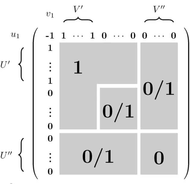
Lastly, suppose that8(u,v)2U@×V@we haveMb0u;v¼0. This case is shown inFig 2.
In addition to the zeroes inU@×V@,Mb0u;v0¼0for anyu2U@. We have jU00j ðm d1Þ
ðu;vÞ 2U00V j Mb0u;v¼0
¼
¼ jU00V00j þ jU00j þ
ðu;vÞ 2U00 ðVnV00n fv0gÞj Mb0u;v¼0
:
ð11Þ
The right-hand side can be estimated from below as follows. Since the row and column sums ofMb0are the same as that ofMX, we have
jU0j c1 Mb0u0;v0¼c1þ1; and jV0j d1 Mb0u0;v0 ¼d1þ1:
For anyv2V0andu2U\U@, we haveMb0u;v¼1. Also, for anyu2U0andv2V\V@, we have Mb0u;v¼1. Therefore
n c1 2 jUnU0n fu0gj jU00j n c2; m d1 2 jVnV0n fu0gj jV00j m d2:
Clearly, ifc2c1+ 1 ord2d1+ 1 (i.e.,Gis almost half-regular), we already have a contra- diction. We also have
ðu;vÞ 2U00 ðVnV00n fv0gÞj Mb0u;v¼0
ðn c2Þðm jV00j 1Þ jUnU0nU00j jVnV0nV00n fv0gj ðn c2Þðm jV00j 1Þ ðn c1 1 jU00jÞ ðm d1 2 jV00jÞ:
ð12Þ
Fig 2.Mb0is shown; each of the entries in the regions marked with 0/1 may be 0 or 1.
https://doi.org/10.1371/journal.pone.0201995.g002
Combining Eqs11and12,
jU00j ðm d1Þ ðn c2Þ ðm jV00j 1Þ þ jU00jðm d1 1Þþ
þ ðjV00j þ1Þ ðn c1 1Þ ðn c1 1Þ ðm d1 1Þ:
Further simplifying:
jU00j ðjV00j þ1Þðc2 c1 1Þ þ ðc1þ1 c2Þmþ ðd1þ1Þn ðc1þ1Þðd1þ1Þ:
Since we may suppose thatc2c1+ 2, we can substitute |V@|m−d2and |U@|n−c1− 2 into the inequality, yielding
ðc2 c1 1Þðd2 d1 1Þ d1ðn c2Þ þ1:
Symmetrically, a similar derivation gives
ðc2 c1 1Þðd2 d1 1Þ c1ðn d2Þ þ1:
The last two inequalities clearly contradict the assumptions of this claim.
In summary, in every case there exist at most 4 switches which transformMb into a 0− 1 matrix, which is a matrix with suitable row- and column sums, therefore it is the adjacency matrix of a realizationKof the degree sequence d.
The analysis of the swap sequences between milestones inM~ Now we turn to discussing the directed case. As in the previous section, condition (O) is the only remaining assumption of Theorem 9 which does not immediately follow from the con- struction of swap sequences between consecutive milestones.
Lemma 12.For any realization Z along the constructed swap sequence from G to G0there exists a realization K=K(Z)such that
d MðXb þY ZÞ;MK
20:
Proof. As described by Lemma 8, it is possible that realizationZis derived by anF-swap which is a firstC4-swap to resolve an alternatingC6cycle along the sweep. It may introduce an extra 2-value and/or a−1-value into the auxiliary structure. But Lemma 8 also shows that the nextC4swap will revert these extra bad positions. Therefore letZSdenote the realizationZitself if this extra swap is not needed, or the new realization if it is needed. ThenMbðXþY ZSÞhas at most two entries of 2 and at most one entry of−1. Now we have to show that there is a reali- zationKsuch that
d MbðXþY ZSÞ;MK
16:
As before we will use the shorthandMbðXþY ZSÞ ¼M:b
The swap sequence transforming the bipartite representationGtoG0(also, the previous extra swap) only touches chords induced byVðCÞ. Therefore, the row and column sums inA[Z] are the same as that ofA[G], so the cornerstone has the minimum row sum inA[Z] as well.
Any entries of 2’s and−1’s inMb are in the row ofu1, moreover, they are contained inA[Z].
SupposeMbu1;v
j ¼2. The column ofvjinA[Z] contains at least one zero, therefore there exist two verticesuk;uk0 2U\VðCÞsuch thatMbuk;vj ¼0andMbu
k0;vj¼0, even if there is ain the column ofvj. We have two cases.
1. There9vl2V\VðCÞsuch thatMbu
k;vl>Mbu1;v
l: obviously,Mbu
k;vl <2, soMbu1;v
l 2 f0; 1g.
The switch operationu1vj,ukvl)u1vl,ukvj(decrease the entries of the matrix by one at positionsu1vjandukvl, and increase the entries at positionsu1vlandukvjby one) inMb (and inA[Z]) eliminates the entry of 2 atu1vj, and creates an entry of 1 at bothu1vjand ukvj. In the columnvlthree scenarios are possible: either the entry−1 and a 0 exchange their positions, or a 0 and a 1 exchange their positions; finally, it is also possible that the−1 and a 1 both become 0.
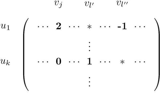
2. If for allvl 2V\VðCÞeitherMbuk;vlMbu1;vlorMbuk;vl ¼ orMbu1;vl ¼ holds: since the sum of the entries in rowu1is minimum among the rows ofA[Z], this is only possible if there existvl0,vl@2V\V(C) such thatMbu1;v
l0 ¼ ,Mbu
k;vl0 ¼1,Mbu1;v
l00 ¼ 1,Mbu
k;vl00 ¼ , and forvl 2V\VðCÞ n fvj;vl0;vl00gwe haveMbu
k;vl¼Mbu1;v
l. This is shown onFig 3.
If the second case applies, the first case must hold if we replacekbyk0; if not, columnvl@
would contain two, a contradiction.
By repeating the previous argument, we may eliminate one more entry 2, if necessary, from A[Z] (andM). (Recall that at the beginning we had at most two 2’s inb M). Although it is possi-b ble that the entry−1 is not in theu1-row anymore, it does not cause any hardship. LetMb0be the matrix we get after performing these at most two switches that eliminate the 2’s. Each entry ofMb0is a 0 or a 1, except at most one−1 entry.
The proof now diverges into two cases corresponding to Theorem 4 and Theorem 5, respectively.
Case of Theorem 4: Sequence d satisfiesEq 4
From now on we will consider the entire matrixMb0and not onlyA. Suppose thatMb0u0;v0¼ 1.
The degrees ofu0andv0are at least one, and so there are at least two entries of 1’s in the row
Fig 3.M is shown for Case 2 of the proof of Lemma 12.b https://doi.org/10.1371/journal.pone.0201995.g003