Article
Remote Sensing of Water Quality Parameters over Lake Balaton by Using Sentinel-3 OLCI
Katalin Blix1,* , Károly Pálffy2, Viktor R. Tóth2and Torbjørn Eltoft1
1 Department of Physics and Technology, UiT the Arctic University of Norway, P.O. Box 6050 Langnes, NO-9037 Tromsø, Norway; torbjorn.eltoft@uit.no
2 Balaton Limnological Institute, Hungarian Academy of Science, Centre for Ecological Research, Klebelsberg K. street 3, 8237 Tihany, Hungary; palffy.karoly@okologia.mta.hu (K.P.); toth.viktor@okologia.mta.hu (V.R.T.)
* Correspondence: katalin.blix@uit.no; Tel.: +47-483-49-399
Received: 23 July 2018; Accepted: 4 October 2018; Published: 11 October 2018 Abstract:The Ocean and Land Color Instrument (OLCI) onboard Sentinel 3A satellite was launched in February 2016. Level 2 (L2) products have been available for the public since July 2017. OLCI provides the possibility to monitor aquatic environments on 300 m spatial resolution on 9 spectral bands, which allows to retrieve detailed information about the water quality of various type of waters.
It has only been a short time since L2 data became accessible, therefore validation of these products from different aquatic environments are required. In this work we study the possibility to use S3 OLCI L2 products to monitor an optically highly complex shallow lake. We test S3 OLCI-derived Chlorophyll-a (Chl-a), Colored Dissolved Organic Matter (CDOM) and Total Suspended Matter (TSM) for complex waters against in situ measurements over Lake Balaton in 2017. In addition, we tested the machine learning Gaussian process regression model, trained locally as a potential candidate to retrieve water quality parameters. We applied the automatic model selection algorithm to select the combination and number of spectral bands for the given water quality parameter to train the Gaussian Process Regression model. Lake Balaton represents different types of aquatic environments (eutrophic, mesotrophic and oligotrophic), hence being able to establish a model to monitor water quality by using S3 OLCI products might allow the generalization of the methodology.
Keywords:shallow lake; Chl-a; CDOM; TSM; Gaussian process regression; automatic model selection algorithm
1. Introduction
Large freshwater lakes play an important role in the earth’s ecosystems, not only because they contain 68% of the global fresh water reservoir, but also because of their economic, social and biological importance as they provide habitats for wildlife, irrigation for agriculture, energy, transport and most importantly water for drinking [1]. The large areal extent of some of these lakes makes traditional water monitoring time and resource consuming, hence inefficient, yet continuous water quality monitoring of lakes is of great importance in detecting environmental changes [2].
Lake Balaton, which covers an area of 596 km2, is the largest lake in Central Europe and one the most important natural and tourist attractions in Hungary and Central Europe. It provides recreational facilities, and is an aesthetics and cultural resort, which attracts the largest tourist industry in the country [3]. There are several ongoing ecosystem monitoring programs at Lake Balaton. These programs aim to monitor important biological and ecological aspects of biodiversity and food web interactions in the lake. Examples for former monitoring programs for Lake Balaton can be found in [4,5].
Water2018,10, 1428; doi:10.3390/w10101428 www.mdpi.com/journal/water
The lake has gone through significant changes in the past decades, and only lately were these changes experienced as advantageous. In the 1970s, increased nutrient loads of anthropogenic origin, such as inadequate wastewater management and agricultural runoff, and abiotic factors resulted in degradation of water quality of Balaton. Anthropogenic impacts, i.e., intensification of agricultural activities and increase in the number of settlements along the shore, caused eutrophication of the lake.
The eutrophication process was successfully stopped and reversed by introducing a combination of technological and management solutions [6,7]. Recent unpublished data suggests that the lake has recovered and returned to the pre-eutrophic conditions.
As a result of these past events, there is an increasing demand for continuous monitoring of biotic and abiotic changes of the lake. Advances in remote sensing technology allow for the use of satellites for monitoring water constituents. The European Space Agency’s (ESA) Ocean and Land Color Instrument (OLCI) onboard the Sentinel 3A and 3B satellites collects data of high spectral and spatial resolutions, and due to the frequent revisit time, they provide the possibility to monitor the water quality of Lake Balaton. In this work, we will study the water monitoring capabilities of Sentinel 3 (S3) for this lake, focusing on three important water quality parameters that affect the lake’s water color through scattering and/or absorption: Chlorophyll-a (Chl-a), Colored Dissolved Organic Matter (CDOM) and Total Suspended Matter (TSM).
Chl-a is a major photosynthetic pigment which occurs in phytoplankton, i.e., in the ubiquitous, microscopic, free-floating and suspended organisms found in the illuminated (euphotic) layer of the lakes. The amount of phytoplankton in the water collectively accounts for the trophic state of the lake. Although these organisms are the base of the aquatic food web, their excess could be harmful.
Phytoplankton face a great number of abiotic and biotic limitations (light, temperature, other algae, herbivores, etc.), which influence the phytoplankton growth [8]. Nutrient enrichment is very important, since it leads to the eutrophication of lakes, which can lead to alternate states [9].
CDOM is the colored (optically active) fraction of the dissolved organic matter (DOM) of waters, consisting mostly of humic and fulvic acids. Although CDOM is considered as an indicator of DOM [10,11], its origin can vary, as the amount of CDOM is affected by external factors and diffuse sources from the catchment. CDOM in waters is autochtonous, i.e., coming from degradation of algae or macrophytes in the given water body, and/or allochtonous, i.e., coming from the catchment area.
TSM includes a wide range of particulate material for the given water column. The origin of TSM can be local, such as wind induced resuspension and/or distant, for instance from tributaries [12].
TSM contains both organic and inorganic matter, and has a significant impact on the spatial and temporal aspects of the optical properties of the water bodies [13].
Ocean color remote sensing methodology could potentially be a useful tool to track the variability and monitor these water quality parameters [14–16]. In situ observations have documented that Lake Balaton shows a large spatial and temporal variation in the amount and the distribution of Chl-a, CDOM and TSM. This, and the fact that Lake Balaton is regularly monitored by field sampling and measurements, makes the lake particularly well suited for validating retrieval of water quality products for complex aquatic environments from the Copernicus S3 OLCI instrument. The computation of the standard Chl-a, CDOM and TSM maps from OLCI is generally performed by using a Neural Network (NN) method [17,18].
However, optical properties of local environments might show large deviations from the data used for training state-of-the-art models. This can lead to erroneous retrieval of water quality parameters [19].
Therefore, it is often required to use a local model, adjusted to the given area. An alternative powerful regression approach, the Gaussian Process Regression (GPR) model, has lately been investigated for biophysical parameter retrieval from remotely sensed data. The GPR model has been shown to outperform some other parameteric and non-parameteric machine learning methods, such as NNs, in the estimation of these biophysical parameters [20–24]. Hence, the GPR model can be an alternative candidate for estimating water quality parameters from data acquired by S3 OLCI in Lake Balaton.
In this work, our primary objective is to investigate the quality of the global S3 OLCI complex water products for Lake Balaton. For this, we compare the OLCI Level 2 (L2) water quality products (Chl-a, CDOM and TSM) against in situ measurements collected at six fixed stations in the lake in 2017.
Hence, the first part of the work is a preliminary study, which aims to investigate the possibility of using S3 OLCI L2 water quality products to monitor Lake Balaton, and at the same time evaluate the performance of S3 OLCI L2 products for this highly complex aquatic environment.
Our secondary objective is to investigate the performance of the Machine Learning GPR approach, tuned locally for Lake Balaton. The GPR model is noted to have several advantageous properties.
In addition to it’s powerful regression strength, it also provides the possibility to access feature relevance, through feature ranking. As shown in [24,25], the regression strength and the efficiency of the model can be improved by using features selected by using ranking methods. In order to select the most suitable number and combination of spectral bands to be used in the GPR model for estimating Chl-a content of Lake Balaton, we applied the recently published Automatic Model Selection Algorithm (AMSA) [25] to data from the lake, extended with synthesised data of the same Chl-a ranges.
Finally, we visually compare the estimates for S3 OLCI L2 Chl-a products with the locally trained GPR model. Note, we do not specifically aim to compare the estimates of the NN with the locally trained GPR model, since the NN was trained on a dataset which differs in optical properties and size from the matchup data we used to train the local GPR model. Hence, our contribution in this work is to test S3 OLCI L2 water quality products for the diverse Lake Balaton conditions, and to comparatively assess the value of using a locally tuned Machine Learning GPR model.
2. Materials and Methods
2.1. Study Area
Lake Balaton is the largest shallow lake in Central Europe, situated in western Hungary (46◦500N, 17◦400 E, Figure1). The surface area of the lake is 596 km2with an average depth of 3.5 m, and the volume is about 2×10⁹m3. Geomorphologically, the lake could be divided into four basins.
One half to two thirds of the inflow is discharged by the main tributary, the Zala River, that enters the lake at the westernmost, Keszthelyi Basin. In past decades, the Zala River has carried a great amount of nutrients into Lake Balaton [26]. This resulted in the deterioration of water quality, mostly in the westernmost, Keszthelyi Basin, which led to a prominent trophic gradient in the lake in the 70s–90s [27]. Although phytoplankton biomass in Lake Balaton has significantly decreased during the last two decades, the trophic gradient along the SW-NE axis still exists.
The northern shore of Lake Balaton is steeper than in the south, which results in a difference in depth between the northern and southern shore. This can allow light to reach the bottom near the southern shore in particular. The bottom of the lake is dominated by fine grain size magnesite-bearing calcareous sediments [28]. This can be easily re-suspended under windy weather conditions, resulting in high turbidity. The spatial variability of algal biomass, bathymetry and bottom sediment content lead to high complexity of the optical properties of Lake Balaton.
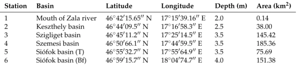
In situ measurements are collected monthly in ice free periods. Six stations are visited, from the westernmost part of the lake, at the outflow of Zala River (Station 1), ending with Station 6 at the easternmost part of the lake (Figure1and Table1). Usually, the data collection is performed at positions assumed to represent typical characteristics of the lake in those areas.
Figure 1.Location of Lake Balaton and the investigated stations.
Table 1.Geographical information of the investigated stations in Lake Balaton.
Station Basin Latitude Longitude Depth (m) Area (km2) 1 Mouth of Zala river 46◦42015.6500N 17◦15039.1600E 2.0 0.14 2 Keszthely basin 46◦44009.500N 17◦16058.300E 2.5 38.00 3 Szigliget basin 46◦45011.200N 17◦25014.500E 3.5 145.42 4 Szemesi basin 46◦50066.100N 17◦44059.500E 3.5 185.36 5 Siófok basin (T) 46◦55032.700N 17◦55064.900E 3.5 75.69 6 Siófok basin (Bf) 46◦59015.700N 18◦04074.700E 4.0 151.38
2.2. Data
2.2.1. Water Sampling
Chlorophyll-a concentration was determined from integrated water samples, which were collected from the whole water column. Water samples of known volume in replicates of 3 were filtered into GF-C filter (Whatman). Chl-a was spectrophotometrically measured after hot methanol extraction [29].
The concentration of CDOM was measured in Pt (platina) units (mg Pt L−1). Water samples of known volume were filtered through a 0.45µm pore size cellulose acetate filter, buffered with borate buffer and measured against a blank of buffered Milli-Q water at 440 nm and 750 nm using a Shimadzu UV 160A spectrophotometer. Pt units were calculated from the absorbance values according to [30].
TSM content was determined gravimetrically after sample filtration through a 0.4µm pore size cellulose acetate filters.
2.2.2. Sentinel-3A OLCI Level-2 Products Water Quality Products
We used the latest reprocessed (14 February 2018) Sentinel-3A OLCI Full Resolution (FR) Level-2 water quality products for complex waters for validation. These products include Chl-a, CDOM and TSM, retrieved from the spectral measurements by using NN techniques. Even though some part of Lake Balaton seems to show oligotrophic conditions, most of the lake is highly complex. Hence, it is reasonable to use water quality products for complex waters retrieved by NN. For further details on the NN retrieval algorithm we refer to [17,18,31].
There were six cloud free images available for the validation study. We located the coordinates of the six stations in the images, and used a 3×3 pixel matrix as described in [32], and applied the
recommended flags. Images were acquired at the days of the in situ measurements or one of the neighboring days. We assume weather conditions were similar. We used the Sentinel Application Platform (SNAP) version 5.0 for processing and preparing the matchups. In total, we could obtain 36 matchups for Chl-a, CDOM and TSM.
We converted the S3 OLCI retrieved CDOM absorbance (m−1) to color (Pt units) by using the expression: Color440(g Pt m−3) = 18.216×a440−0.209 [30,33].
Remote Sensing Reflectance (Rrs)
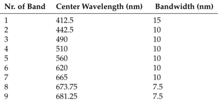
We have also extracted the Level-2 Rrs for the spectral bands summarized in Table2, by following the same procedure as described above. This data was included in the dataset used for training and testing the alternative GPR approach to retrieve the Chl-a water quality parameter.
Table 2.Summary of the Sentinel 3A OLCI spectral bands.
Nr. of Band Center Wavelength (nm) Bandwidth (nm)
1 412.5 15
2 442.5 10
3 490 10
4 510 10
5 560 10
6 620 10
7 665 10
8 673.75 7.5
9 681.25 7.5
2.2.3. Synthetic Dataset
An additional synthetic dataset was generated by using HydroLight simulation. The dataset includes Chl-a concentrations over a wide range, with corresponding Rrs values of the S3 OLCI bands. We extracted the values corresponding to the ranges of in situ Chl-a measurements from Lake Balaton. This dataset was used for evaluating the alternative model to estimate Chl-a concentration in Lake Balaton.
2.3. Methodology
2.3.1. Statistical Analysis
We evaluated the S3 OLCI products by comparing the retrieved values to in situ measurements of Chl-a, CDOM and TSM, respectively. For each water quality parameter, we quantified the correspondence in terms of three statistical measure. These measures are the Bias, the Normalized Root Mean Squared Errors (NRMSE), and the Squared Correlation Coefficient (r2). They are defined by:
Bias= 1 N
∑
N i=1|(yi−yˆi)|, (1)
NRMSE= 1
ymax−ymin v u u t1
N
∑
N i=1(yi−yˆi)2, (2)
r2= ∑
N
i=1(yˆi−y)2
∑i=1N (yi−yi)2, (3) whereNis the number of observations,yis the in situ measurement, ˆyis the S3 OLCI product,ymaxis the maximum observed value,yminis the minimum observed value, andyis the mean of the in situ measurements. We have also computed thep-value for assessing the level of significance. Thep-value ranges between 0 and 1. A lowp-value indicates that the null-hypothesis, which states there is no
relationship between the results and the data, can be rejected. The cut off value is user-defined, and usually set to 0.05. Hence ap-value < 0.05, means that the results are significant, while ap-value > 0.05 indicate little or no significance.
2.3.2. Machine Learning Gaussian Process Regression for Water Quality Estimation GPR Model
Machine Learning by Gaussian Process Regression (GPR) has been demonstrated to perform excellently in the prediction of water quality parameters from remotely sensed data [20,21,23,24].
Therefore, we have chosen to evaluate this methodology on the matchup data obtained for Lake Balaton in 2017.
The GPR model is a flexible, non-linear kernel method, which learns the functional relationship between the input and output by using a Bayesian framework [34]. In this work, the input data ({xn ∈RD}Nn=1) is formed by using the spectral bands from S3 OLCI Rrs (Table2), wheren=1, ...,N is the number of measurements, andd=1, ...,Dis the number of spectral bands. The output (yn=1N ) is thein situand synthetic measurements for Chl-a.
The functional relationship between the input and output can be written byyn = f(xn) +εn, for n = 1, ...,N, where the noise term, εn, is assumed to be additive, independently, identically Gaussian distributed, with zero mean and constant variance, i.e.,εn ∼ N(0,σ2). The GPR model fits a multivariate joint Gaussian distribution over the function values f(x1), ...,f(xN) ∼ N(0,K), with zero mean and covariance matrixK. Using a Bayesian inversion, the posterior distribution can be analytically computed for the predicted output (y∗) for the corresponding new input (x∗).
This can be written byp(y∗|x∗,D) =N(y∗|µGP∗,σGP∗2 ), whereµGP∗is the predicted Chl-a,σGP∗2 is the certainty level of the estimate, andDis the training data. The predicted Chl-a can be expressed by µGP∗=k>∗(K+σ2In)−1y, wherek>∗ is the transposed covariance between the training vector and the test point. For further details on the GPR model we refer to [34].
Automatic Model Selection Algorithm
We used the Automatic Model Selection Algorithm (AMSA), described in [25], to determine the most suitable Chl-a retrieval GPR model for Lake Balaton. AMSA uses feature ranking methods to select the combination of features that results in the strongest regression, based on some predefined quantitative regression performance measures.
Since different ranking methods, may rank the features differently, we used four feature ranking methods here. These are the Sensitivity Analysis (SA) of the GPR and Support Vector Regression (SVR) models, the Automatic Relevance Determination (ARD), and the Variable Importance in Projection (VIP).
For each station, the spectral bands were ranked by these four methods. Then the ranked bands were fed into the GPR model to perform regression, starting with the most relevant band, then the second most important band, and subsequently, the next ranked bands in decreasing order of importance. At each iteration, regression performance measures are computed, and used for evaluating the strength of the GPR with the combination of features. The computation is done until no further improvement is achieved, and is repeated for all the four sets of ranked spectral bands resulting from the SA GPR, SA SVR, ARD and VIP feature ranking methods. This process was done for each station.
Machine Learning GPR for Lake Balaton
We had six matchups available for each of the stations. These matchups were merged with synthetic data of the corresponding Chl-a contents. This allowed us to obtain a larger representative dataset. We used the procedure described above to determine a ’best’ GPR model, i.e., a best spectral combination for each station. The purpose of this exercise was to assess if the GPR model is spectrally sensitive to the observed changes in the water conditions.
We also wanted to find a ’best’ GPR model for the whole Lake Balaton. Hence, in order to find a GPR model that generalizes best for the whole lake, each of the station-wise ’best’ models was next trained and tested on the whole data set. The training and testing were done by carrying out cross validation in 500 iterations. We also evaluated the GPR model using all spectral bands in the input vector.
3. Results
3.1. Data Acquisition
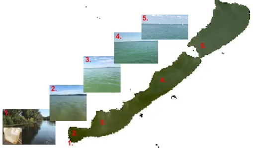
The optical properties of the stations show great spatial and temporal variation. Station 1 is rich in CDOM, hence the color of the water appears dark-brown, while stations 5 and 6 are usually oligotrophic, resulting in blue water color, similarly to open oceans. Figure2shows an RGB image acquired in August 2017 by S3 OLCI, supplemented by photos taken at the stations, when the corresponding sampling was carried out. As can be clearly observed the color of the water is changing from station to station.
Figure 2.Color gradient in Lake Balaton. The RGB image was acquired by S3 OLCI at 18 August 2017, and the photos were taken at the stations, while the corresponding is situ measurements were collected.
3.1.1. In Situ Measurements
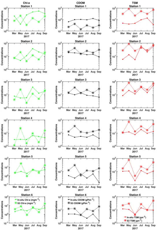
Table3summarizes the results of the in situ measurements for every month and station. It can be observed that every month shows large spatial variation in all water quality parameters. More details of these variations are depicted in Figure6, where the temporal variations of the water quality parameters at each station, together with the S3 OLCI L2 products, are presented. Note that the temporal variations at the stations seem to show differences between the measured parameters. In case of Chl-a, stations 1, 2 and 3 have the largest variations, while stations 4, 5 and 6 have quite steady values. The range of CDOM concentration decreases from station 1 to 6, following the trophic gradient of the lake.
For most of the measurements, we can disregard the contribution of bottom reflectance to the measured signal, since the depth of the euphotic zone does not reach the bottom. However, there were three measurements (in June at station 5 and 6, and in August at station 5), which might include contribution from bottom reflectance. This presumption based on evaluation of the respective computed light extinction coefficients.
Table 3. Summary of the range of thein situmeasured water quality parameters in 2017. See also Figure6for further representation of the variablility of the water quality parameters for every station.
Monthly Range
Month Chl-a (mg m−3) CDOM (g Pt m−3) TSM (g m−3)
March 2–20 5–64 5–11
May 3–6 3–100 4–21
June 2–25 4–103 2–12
July 5–46 2–95 12–61
August 3–55 5–124 7–21
September 5–33 2–84 4–60
Station Wise Range
Station Chl-a (mg m−3) CDOM (g Pt m−3) TSM (g m−3)
1 4–55 64–124 4–14
2 5–38 9–19 6–60
3 6–38 6–14 9–51
4 3–6 4–7 8–14
5 2–5 2–7 2–12
6 2–5 2–5 5–15
3.1.2. Satellite Products
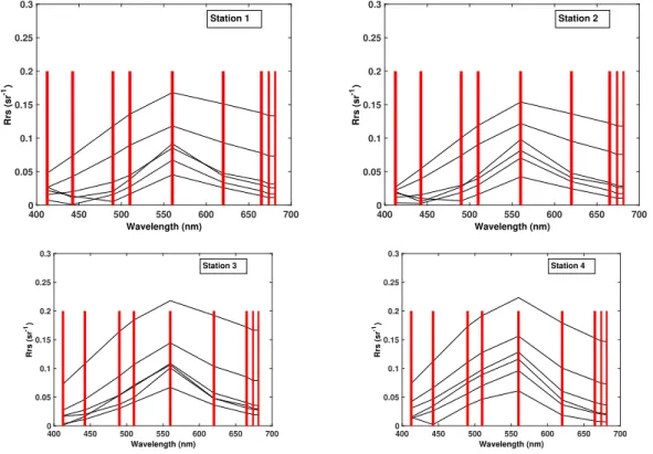
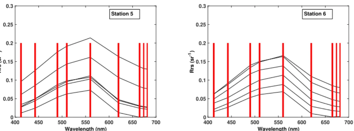
Figure3 shows the Rrs values of the six stations. It can be observed that the CDOM rich stations show a greater variation in the spectrum (Figure3top-row) than stations with low CDOM concentrations (Figure3bottom-row). This may be explained by the overlapping absorption spectra of Chl-a and CDOM. It might also be a result of the higher Chl-a concentration in itself, since stations with higher CDOM also have higher Chl-a in general. Station 1 and 2 have similar spectra, they are comparable in terms of Chl-a, but they significantly differ in CDOM (and in TSM too) concentration.
400 450 500 550 600 650 700
Wavelength (nm) 0
0.05 0.1 0.15 0.2 0.25 0.3
Rrs (sr-1)
Station 1
400 450 500 550 600 650 700
Wavelength (nm) 0
0.05 0.1 0.15 0.2 0.25 0.3
Rrs (sr-1)
Station 2
400 450 500 550 600 650 700
Wavelength (nm) 0
0.05 0.1 0.15 0.2 0.25 0.3
Rrs (sr-1)
Station 3
400 450 500 550 600 650 700
Wavelength (nm) 0
0.05 0.1 0.15 0.2 0.25 0.3
Rrs (sr-1)
Station 4
Figure 3.Cont.
400 450 500 550 600 650 700 Wavelength (nm)
0 0.05 0.1 0.15 0.2 0.25 0.3
Rrs (sr-1)
Station 5
400 450 500 550 600 650 700
Wavelength (nm) 0
0.05 0.1 0.15 0.2 0.25 0.3
Rrs (sr-1)
Station 6
Figure 3.S3 retrieved Rrs values for the 9 spectral bands at the 6 stations. The red bars indicate the position of the bands, and their widths illustrate the relative proportion of the width of the bands.
3.2. Validation
First, we compared the in situ measurements with the S3 OLCI-derived products for all the available data. This allowed us to have an overall understanding about the accuracy of the estimation of the parameters.
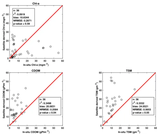
Figure4shows the correspondence between the histograms of the S3 products and the in situ measurements. It can be observed that for the Chl-a (Figure4top) the histograms show similar and overlapping distributions of the estimated values. However, there are no satellite-derived estimates above 30 mg m−3. In case of CDOM (Figure4bottom-left), the histograms also reveal similar distributions, although the satellite estimates are shifted to higher values. Furthermore, the satellite estimates could not capture values above 50 g Pt m−3. The histograms of the TSM concentrations (Figure4bottom-right) show little agreement. Satellite estimates have a more uniform spread, with a significant shift towards higher values, compared to the in situ measurements.
Figure 5 shows scatter-plots of the measured in situ water quality parameters versus the corresponding satellite-derived products for all stations. It can be observed that in case of the Chl-a content (Figure5top), the S3 OLCI Chl-a retrieval algorithm does not estimate concentrations above 30 mg m−3. The opposite of this tendency can be seen for the CDOM (Figure5bottom-left) and TSM (Figure5bottom-right) concentrations. The satellite products show significantly higher values than the in situ measurements.
With reference to Figure 5, the corresponding r2 measure showed no correlation for Chl-a, but some correlation for CDOM and TSM. However, the lowest bias was computed for Chl-a, while both for CDOM and TSM the bias were higher. Finally, the NRMSE values were similar for Chl-a and CDOM, and higher for TSM.
In order to detect both monthly and station wise variations in the estimation of water quality products by using S3 OLCI, we compared the in situ measurements with the L2 products for every station and month. The results of the computed statistical measures can be seen in Tables4and5.
Figure 4.Histogram of the in situ and satellite-derived (S3) water quality concentrations: Chl-a (top), CDOM (bottom-left) and TSM (bottom-right).
0 10 20 30 40 50 60
In-situ Chl-a (mgm-3) 0
10 20 30 40 50 60
Satellite derived Chl-a (mgm-3)
Chl-a
n: 36 r2: 0.0919 bias: 10.6344 NRMSE: 0.2871 p-value = 0.59
0 10 20 30 40 50 60
In-situ CDOM (gPtm-3) 0
10 20 30 40 50 60
Satellite derived CDOM (gPtm-3)
CDOM
n: 36 r2: 0.3498 bias: 20.0831 NRMSE: 0.2584 p-value = 0.04
0 10 20 30 40 50 60
In-situ TSM (gm-3) 0
10 20 30 40 50 60
Satellite derived TSM (gm-3)
TSM
n: 36 r2: 0.3332 bias: 24.0521 NRMSE: 0.5653 p-value = 0.05
Figure 5.In situ versus satellite-derived water quality concentrations: Chl-a (top), CDOM (bottom-left) and TSM (bottom-right).
Station Wise Analysis
Analyzing the computed statistical measures station-wise revealed poor correspondence between the satellite retrievals and in situ measurements for all water quality parameters (Table4). Stations 6 and 5 seemed to show the best values for S3 OLCI Chl-a and CDOM retrieval, respectively. These stations correspond to the area where both Chl-a and CDOM concentrations are low (Table3). For the estimated TSM concentration, station 3 seemed to show the best computed statistical measures.
In order to visually assess the temporal variations of the water quality parameters at the stations, we have depicted the in situ measurements and the S3 OLCI-derived values for every station in Figure6.
It can be seen that Chl-a is underestimated for stations 1, 2 and 3, with the exception of the May month. For stations 4, 5 and 6 S3 the OLCI algorithm both over- and underestimates Chl-a content. However, these biases seem to decrease as in situ Chl-a content decreases and shows less variations. CDOM is overestimated almost at all stations, with the exception of station 1, where it is underestimated for all months. The TSM concentration is also overestimated at all stations. The largest deviation seems to occur at station 1, while the smallest difference occurs at station 3. This is in good agreement with the computed statistical measures.
Table 4.Validation results: summary of the computed measures for the water quality parameters for every station.
Chl-a
Station NRMSE Bias r2 p-Value
1 0.5405 24.5915 0.1538 0.442
2 0.4326 11.6173 0.0200 0.789
3 0.4311 10.6361 0.0104 0.847
4 3.0461 6.9700 0.0026 0.92
5 3.1640 6.1978 0.0863 0.571
6 1.6021 3.7935 0.4163 0.166
CDOM
Month NRMSE Bias r2 p-Value
1 1.1985 68.0526 0.0290 0.747
2 1.4492 11.3669 7.3−4 0.959
3 1.9824 11.4616 0.2600 0.301
4 4.2534 11.2679 0.1297 0.483
5 2.7703 10.9008 0.3768 0.195
6 2.6877 7.4488 0.2942 0.266
TSM
Month NRMSE Bias r2 p-Value
1 5.0034 42.8140 0.1322 0.478
2 0.6156 25.4804 0.1138 0.51
3 0.6311 18.8408 0.4160 0.166
4 2.6384 20.5351 0.1662 0.42
5 3.2746 22.4133 0.3522 0.21
6 2.0486 14.2292 0.1731 0.41
Mar May Jun Jul Aug Sep 2017
100 101 102
Concentrations
Chl-a Station 1
Mar May Jun Jul Aug Sep 2017
101 102 103
Concentrations
CDOM Station 1
Mar May Jun Jul Aug Sep 2017
100 101 102
Concentrations
TSM Station 1
Mar May Jun Jul Aug Sep 2017
100 101 102
Concentrations
Station 2
Mar May Jun Jul Aug Sep 2017
100 101 102
Concentrations
Station 2
Mar May Jun Jul Aug Sep 2017
100 101 102
Concentrations
Station 2
Mar May Jun Jul Aug Sep 2017
100 101 102
Concentrations
Station 3
Mar May Jun Jul Aug Sep 2017
100 101 102
Concentrations
Station 3
Mar May Jun Jul Aug Sep 2017
100 101 102
Concentrations
Station 3
Mar May Jun Jul Aug Sep 2017
100 101 102
Concentrations
Station 4
Mar May Jun Jul Aug Sep 2017
100 101 102
Concentrations
Station 4
Mar May Jun Jul Aug Sep 2017
100 101 102
Concentrations
Station 4
Mar May Jun Jul Aug Sep 2017
10-1 100 101 102
Concentrations
Station 5
Mar May Jun Jul Aug Sep 2017
100 101 102
Concentrations
Station 5
Mar May Jun Jul Aug Sep 2017
100 101 102
Concentrations
Station 5
Mar May Jun Jul Aug Sep 2017
10-1 100 101 102
Concentrations
Station 6 In-situ Chl-a (mgm-3) S3 Chl-a (mgm-3)
Mar May Jun Jul Aug Sep 2017
100 101 102
Concentrations
Station 6 In-situ CDOM (gPtm-3) S3 CDOM (gPtm-3)
Mar May Jun Jul Aug Sep 2017
100 101 102
Concentrations
Station 6
In-situ TSM (gm-3) S3 TSM (gm-3)
Figure 6.In situ versus satellite-derived water quality products for the stations. Chl-a is shown in the left panel, CDOM in the middle, and TSM in the right panel. Y-axis is presented on a logarithmic scale.
Monthly Analysis
Analyzing the data for each month revealed that the poorest performance was obtained in May for all the three parameters (Table5). This might be related to the mixing of the water layers, which may cause the sensitivity of the NN algorithm to be biased towards the TSM. However, the computed biases were large for all months and parameters. The highest agreement between in situ observations and S3 OLCI products were found for the Chl-a concentration, with the exception for May. The computed correlation coefficients were found to be low for both the CDOM and TSM concentrations for most of the months.
Table 5.Validation results: summary of the computed measures for the water quality parameters for each month.
Chl-a
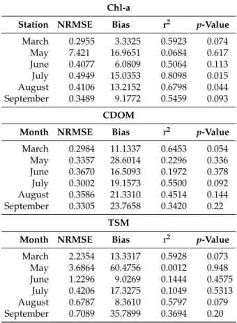
Station NRMSE Bias r2 p-Value March 0.2955 3.3325 0.5923 0.074
May 7.421 16.9651 0.0684 0.617 June 0.4077 6.0809 0.5064 0.113 July 0.4949 15.0353 0.8098 0.015 August 0.4106 13.2152 0.6798 0.044 September 0.3489 9.1772 0.5459 0.093
CDOM
Month NRMSE Bias r2 p-Value March 0.2984 11.1337 0.6453 0.054
May 0.3357 28.6014 0.2296 0.336 June 0.3670 16.5093 0.1972 0.378 July 0.3002 19.1573 0.5500 0.092 August 0.3586 21.3310 0.4514 0.144 September 0.3305 23.7658 0.3420 0.22
TSM
Month NRMSE Bias r2 p-Value March 2.2354 13.3317 0.5928 0.073
May 3.6864 60.4756 0.0012 0.948 June 1.2296 9.0269 0.1444 0.4575
July 0.4206 17.3275 0.1049 0.5313 August 0.6787 8.3610 0.5797 0.079 September 0.7089 35.7899 0.3694 0.20
3.3. GPR for Lake Balaton Chlorofyll: A Content Retrieval
The validation results above indicate that there is a need for a local model in the estimation of water quality parameters over Lake Balaton based on S3 OLCI data. Therefore, in the following section we present the results of a locally tuned GPR model for Chl-a content.
3.3.1. AMSA for Improving the GPR Model for Chl: A Content Retrieval
We used AMSA to determine the number and positions of the most important spectral bands for the six stations for Chl-a. This was done by extracting the Chl-a and Rrs pairs from the synthetic dataset corresponding to the in situ Chl-a ranges for every station. Then the synthetic dataset was merged with the in situ data. This was used as input to AMSA. Then the first stage of AMSA, feature ranking, was done by using all the available samples (Table6Nr. of samples) for each station. The feature selection and evaluation part of AMSA were performed by splitting the data to training and testing samples. The test samples were formed by the in situ measurements, while the training samples held the rest of the samples. Table6summarizes the results for the stations. Thep-value was below 0.0001 for all cases. Note, the results in Table6show the strongest models for the stations. However, using only few ranked bands as input to the GPR model already resulted in strong performance. The goal is to determine the ’best’ model, therefore, these results are not reported here.
Table 6.Summary of the stationwise evaluation of AMSA for Chl-a for the merged dataset.
Station Nr. of Samples Nr. of Bands NRMSE r2
1 769 8 0.0187 0.9995
2 675 6 0.0653 0.9984
3 646 9 0.0273 0.9988
4 784 5 0.0187 1.0000
5 695 6 0.0501 0.9979
6 745 3 0.0657 1.0000
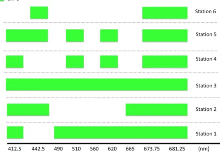
The spectral bands needed to achieve the ’best’ GPR model are summarized in Figure7. It can be observed that for all stations, bands centered at 673.25 and 681.25 nm were needed to obtain the strongest regression for Chl-a content estimation in the GPR model. For station 6, using only three bands were already enough to determine the ’best’ model. These three bands are centered at 442.5, 673.75 and 681.25 nm, which is in good correspondence with the Chl-a absorption and fluorescence spectrum. Station 6 is known to be less affected by CDOM, hence possibly the first absorption peak of Chl-a is not masked by CDOM.
Figure 7.The most important spectral bands of Chl-a for each station.
3.3.2. Determining a General Model for Chl-a Content Retrieval
We used the results of the station-wise feature ranking from AMSA to determine a general GPR model tuned for the whole lake. Firstly, we used all the available spectral bands in the GPR model.
This was defined as our reference model. Then we used the results of the ranking methods presented in Figure7for the stations to perform regression experiment involving the complete merged dataset.
Table7shows the computed statistics for the GPR models. Note that for Station 3, AMSA suggested that all bands were needed. All stations considered, the general observation was that the lowest bias was achieved by using bands centered at 412.5, 510, 620, 673.75 and 681.25 nm, and the lowest NRMSE was obtained with the bands centered at 442.5, 673.75 and 681.25 nm. Hereafter, we refer to these models as the all bands, the 5-band and the 3-band models, respectively, Thep-value, which was very low in all cases, and r2measure could not reveal any differences between the models.
Table 7. Summary of the computed statistical measures for the six GPR models. Thep-value was significantly below 0.0001 for all cases.
Station Bands Used in the GPR Model NRMSE Bias r2
All 0.00448 0.2056 1.0000
1 1, 3, 4, 5, 6, 7 and 8 0.0046 0.2047 1.0000
2 1, 2, 6, 7 and 8 0.0047 0.2037 1.0000
3 All 0.00448 0.2056 1.0000
4 1, 4, 6, 8 and 9 0.0031 0.1351 1.0000
5 1, 2, 4, 6, 8 and 9 0.0034 1.1414 1.0000
6 2, 8 and 9 0.003 0.1365 1.0000
3.3.3. Cross Validation
We used all bands, 5-band and 3-band models to perform cross-validation. For this purpose, we merged the synthetic and in situ data for all stations. In order to reduce computational time we used a subset of this merged dataset. This data was formed by sampling from the values from every station, hence the data was still representative for the whole lake. The total number of samples were 624.
We used this representative dataset to randomly draw samples from both the synthetic and in situ measurements for training the models, while the rest of the data was used for testing. The total number of samples used for training and testing, was 430 and 194, respectively. Then we computed the statistical measures on the test set. This was done for 500 times. The results are summarized in Table8. It can be seen that both the 5-band and 3-band models resulted in improved performance in comparison to the all band model. The lowest NRMSE and bias were achieved by the 5-band model, and the highest r2was obtained with the 3-band model. Thep-value were low in all cases. Note, both models include bands centered at 673.75 and 681.25 nm. These results confirm the importance of using these bands to estimate Chl-a in optically highly complex waters.
Table 8.Summary of the cross validation. The results show the mean values of the NRMSE, Bias, r2 andp-value by using the GPR model with all bands, 5-bands and 3-band models for 500 iterations.
GPR Model NRMSE Bias r2 p-Value All bands 0.1136 2.2532 0.7909 <0.0001 5-bands 0.1042 2.0563 0.8253 <0.0001 3-bands 0.1043 2.1247 0.8298 <0.0001
3.3.4. Chl-a Maps
By comparing the satellite products with the ground-truth measurements for all months, revealed that May had the largest deviations according to the statistical measures for all water quality parameters (Table5).
The RGB image of Lake Balaton acquired at the 22 May 2017 can be seen in Figure8. The yellowish pattern are most likely due to the mixing of the bottom layers. These patterns show good correspondence with the dominating wind direction, Northern winds, and the geography of the Northern shore of the lake. Note, the patches, which appear green in the image, are in areas well-known to be shadowed for the Northern winds.
Figure9shows the estimated Chl-a content by using S3 OLCI NNs (left) and the 5-band GPR model (right). It can be observed that the S3 OLCI product overestimates Chl-a content. This might be due to a too strong sensitivity to TSM. Comparing the RGB image and the Chl-a estimates-derived by S3 OLCI, we see that it follows the pattern of thoroughly mixed waters with higher TSM. the 5-band GPR model seem to show less (no) sensitivity to the TSM concentration. Chl-a estimates show higher values in the western basin, around the Tihany passage and also around the eastern basin. Fine details and patterns can also be observed in the image produced by the 5-band GPR model.
Patches with higher Chl-a content seem to appear in areas, where the primary productivity is assumed to be increased. The map (Figure9right) revealed regions with higher Chl-a values, in the western and eastern side of the Tihany passage. This is an interesting feature, which can be explained by the bathymetry of the lake. The water depth drops around the southern part of the passage [35,36], allowing benthic algae to appear in surface waters under suitable mixing conditions. The RGB image showed heavy mixing in the particular month we chose for this illustration. Favorable wind direction and speed might have caused the occurrence of a current in the Tihany passage, transporting Chl-a rich waters from the western part to the eastern side.
Figure 8.The RGB image of Lake Balaton at the 22 May 2017.
0 5 10 15 20 25 30
0 5 10 15 20 25 30
Figure 9. Chl-a content estimates by S3 OLCI (left) and the 5-band GPR (right). The units are in mg m−3.
4. Discussion
In this work, we studied the possibility of using S3 OLCI L2 products to monitor water quality parameters in Lake Balaton. For this, we first used in situ measurements of Chl-a, CDOM and TSM to evaluate the performance of the state-of-the-the-art complex water algorithm for S3 OLCI. The overall finding was that the correlation between in situ measurements and the S3 OLCI L2 products was low and not significant. It was the lowest value for Chl-a content, and somewhat higher for CDOM and TSM. Note, there are few published validation results for S3 OLCI L2 water quality parameters for complex waters, since S3 OLCI data only lately has become available. However, for the MEdium Resolution Imaging Spectrometer (MERIS), which had similar spectral and spatial resolution as S3 OLCI, similar validation results have been documented using NN algorithms to retrieve water quality parameters. This includes the over and underestimation of Chl-a concentration [37], and large overestimation of TSM [31].
The station-wise study resulted in the best qualitative correspondence, i.e., lowest NRSME and bias, and highest correlation, for Chl-a and CDOM at stations representing oligotrophic waters (Stations 5 and 6). The range of the in situ measurements at these stations were between 2 and 5 mg m−3 for Chl-a and 2–7 g Pt m−3for CDOM, which are the lowest of all stations. Here, the TSM concentrations were also in the lower ranges, in comparison to the other stations. The computed measures did not reveal any significant differences between the stations for TSM.
The monthly analyses showed that the S3 OLCI estimates were in quite good correspondence with the observations for Chl-a. CDOM and TSM estimates had less agreement with the in situ measurements.
We found that May resulted in the poorest fit in terms the computed statistical measures. The in situ Chl-a ranges were lowest in May, but conversely, for this month the CDOM and TSM ranges were large.
These results might be related to inaccuracies in the atmospheric correction and water quality retrieval algorithms because of the lack of training data from Lake Balaton in the dataset used to establish the state-of-the-the-art models for complex waters [38].
The above results motivated us to investigate the capabilities of a locally trained GPR model for monitoring the complex environment of Lake Balaton. The overall findings for the S3 OLCI products showed the poorest performance for Chl-a content retrieval, which is the most important water quality parameter. Therefore, we studied the possibility of improving Chl-a content estimation in Lake Balaton by using the alternative approach. We obtained a larger, more representative dataset suitable for evaluating a locally tuned model by extending the in situ measurements with a synthetic dataset for S3 OLCI, generated for complex waters.
Using the AMSA approach to determine the most suitable number and combination of spectral bands to be used in the GPR model, we obtained significant improvements in regression strength.
Even though the four feature ranking methods currently implemented in AMSA are-derived from different mathematical principles, the ranking showed high consistency. Our station-wise feature ranking experiment showed that the most relevant bands were highly dependent of the water properties and the water quality parameter in question. Our study suggested that for Chl-a estimation in Lake Balaton the bands 1, 4, 6, 8 and 9 are the most important in the GPR model. These bands have been previously shown to be sensitive to Chl-a in different datasets [24]. Bands positioned in the red part of the electromagnetic spectrum, corresponding to the longer wavelengths, might be important due to the second absorption peak of the Chl-a molecule [39]. Recent studies have presented the benefit of using S3 OLCI red bands to monitor Chl-a in optically complex environments [40,41]. Chl-a estimation can be improved by using models with these red bands. This is in good correspondence with our results. The station-wise analysis of AMSA showed that inclusion of red bands were necessary to obtain the ’best’ GPR model for all cases. The 5-band model for Lake Balaton also was found to use these red bands as inputs to achieve improved Chl-a retrieval. The inclusion of additional blue-green bands has been shown to be advantageous, when the aquatic environment has large variation in Chl-a content [42]. Our results also indicated that bands corresponding to lower relative wavelengths are also required to optimize the GPR model for the lake.
We visually compared the predictive power of the locally tuned 5-band GPR model with S3 OLCI L2 Chl-a products for Chl-a estimation. The Chl-a map produced by using S3 OLCI L2 NN algorithm seemed to show high sensitivity to the TSM content. The estimated Chl-a contents were significantly above the in situ measurements, indicating overestimation. This is in good agreement with the validation results, which showed that S3 OLCI assigns high values to Chl-a content below about 10 mg m−3. This is a surprising finding, since the state-of-the-the art NN was trained on samples containing values up to 30 mg m−3. A possible explanation for this overestimation is that complex optical properties of the lake results in sensitivity to other water constituents, such as TSM. This might lead to erroneous Chl-a content estimates. This also suggests the importance of using an alternative flexible approach for local, highly complex aquatic environment. The Chl-a map produced by the 5-band GPR model seemed to show better correspondence with the measured Chl-a content range for
the particular month. The model could capture fine details and patches, which can be explained by the bathymetry and currents in the lake.
5. Conclusions
Our analysis showed that S3 OLCI provides the excellent possibility to monitor Lake Balaton, due to its spectral and spatial resolution and the good quality of the data. However, our validation results indicate the need of algorithm development for optically highly complex waters. We can conclude that based on the evaluation study of the alternative approach on the composite dataset, the GPR model seems to be able to improve the estimation of Chl-a concentration in Lake Balaton.
We believe that the development of an accurate, fast and robust water quality retrieval model for Lake Balaton would certainly be generally beneficial. This is due to the fact that Lake Balaton’s optical properties represent different kinds of aquatic environments: eutrophic, mesotrophic, oligotrophic, turbid and clear waters, and possible contribution of bottom reflectance. Hence, the lake represents a unique test site for the development of retrieval models for water quality parameters for optically complex waters.
For future work, we will collect in situ radiometric data, which might allow to further exploit the optical properties of Lake Balaton and understand eventual challenges with regard to the atmospheric correction algorithm. Furthermore, we will further test and validate the alternative model presented here on data originating from various other water bodies. This might allow us to understand the generalization capabilities of the 5-band GPR model.
Author Contributions:K.B. conceived the idea, methodology, performed the implementations, validation, formal analysis, data processing and analysis, visualization and prepared the original draft. K. P., V. R. T. and T. E.
contributed to the investigation, interpretation of the results, writing-review and editing. T. E. supervised the work.
Funding:This research received no external funding.
Acknowledgments: This research is partly funded by CIRFA partners and the Research Council of Norway (grant number 237906). We thank the Hungarian Academy of Science, Center for Ecological Research, Balaton Limnological Institute for providing the data, and to Balázs Németh for his useful comments and discussions.
We thank EUMETSAT for producing and distributing the S3 OLCI L2 data. We thank Nima Pahlevan (National Aeronautics and Space Administration/Goddard Space Flight Center) for providing the synthetic dataset.
Conflicts of Interest:The authors declare no conflict of interest.
References
1. Beeton, A.M. Large freshwater lakes: Present state, trends, and future. Environ. Conserv.2002,29, 21–38.
[CrossRef]
2. Palmer, S.; Zlinszky, A.; Balzter, H.; Perea, V.N.; Tóth, V. Copernicus Framework for Monitoring Lake Balaton Phytoplankton. InEarth Observation for Land and Emergency Monitoring; Wiley-Blackwell: Hoboken, NJ, USA, 2017; Chapter 10, pp. 173–191. [CrossRef]
3. Rátz, T.; Michalkó, G.; Kovács, B. The influence of Lake Balaton’s tourist milieu on visitors’ quality of life.
Tourism Int. Interdiscip. J.2008,56, 127–142.
4. Mózes, A.; Présing, M.; Vörös, L. Seasonal Dynamics of Picocyanobacteria and Picoeukaryotes in a Large Shallow Lake (Lake Balaton, Hungary). Int. Rev. Hydrobiol.2006,91, 38–50. [CrossRef]
5. Riddick, C.A.L.; Hunter, P.D.; Tyler, A.N.; Martinez-Vicente, V.; Horváth, H.; Kovács, A.W.; Vörös, L.;
Preston, T.; Présing, M. Spatial variability of absorption coefficients over a biogeochemical gradient in a large and optically complex shallow lake. J. Geophys. Res. Oceans2015,120, 7040–7066. [CrossRef]
6. Somlyódy, L.; van Straten, G. Background to the Lake Balaton Eutrophication Problem. InModeling and Managing Shallow Lake Eutrophication with Application to Lake Balaton; Springer: Berlin, Germany, 1986;
pp. 3–18.
7. Istvánovics, V.; Clement, A.; Somlyody, L.; Specziár, A.; László, G.; Padisak, J. Updating water quality targets for shallow Lake Balaton (Hungary), recovering from eutrophication. Hydrobiologia2007,581, 305–318.
[CrossRef]
8. Reynolds, C.S.; Scheiz, Z. The response of phytoplankton communities to changing lake environments.
Swiss J. Hydrol.1987,49, 220–236. [CrossRef]
9. Scheffer, M.; Hosper, S.; Meijer, M.L.; Moss, B.; Jeppesen, E. Alternative equilibria in shallow lakes.
Trends Ecol. Evol.1993,8, 275–279. [CrossRef]
10. Brezonik, P.L.; Olmanson, L.G.; Finlay, J.C.; Bauer, M.E. Factors affecting the measurement of CDOM by remote sensing of optically complex inland waters. Remote Sens. Environ.2015,157, 199–215. [CrossRef]
11. Toming, K.; Kutser, T.; Tuvikene, L.; Viik, M.; Nõges, T. Dissolved organic carbon and its potential predictors in eutrophic lakes. Water Res.2016,102, 32–40. [CrossRef] [PubMed]
12. Madsen, J.D.; Chambers, P.A.; James, W.F.; Koch, E.W.; Westlake, D.F. The interaction between water movement, sediment dynamics and submersed macrophytes. Hydrobiologia2001,444, 71–84.:1017520800568.
[CrossRef]
13. Giardino, C.; Oggioni, A.; Bresciani, M.; Yan, H. Remote Sensing of Suspended Matter in Himalayan Lakes.
Mt. Res. Dev.2010,30, 157–168, doi:10.1659/MRD-JOURNAL-D-09-00042.1. [CrossRef]
14. Büttner, G.; Korándi, M.; Gyömörei, A.; Köte, Z.; Szabó, G. Satellite remote sensing of inland waters:
Lake Balaton and reservoir Kisköre. Acta Astronaut.1987,15, 305–311. [CrossRef]
15. Palmer, S.C.; Hunter, P.D.; Lankester, T.; Hubbard, S.; Spyrakos, E.; Tyler, A.N.; Présing, M.; Horváth, H.;
Lamb, A.; Balzter, H.; et al. Validation of Envisat MERIS algorithms for chlorophyll retrieval in a large, turbid and optically-complex shallow lake. Remote Sens. Environ.2015,157, 158–169. [CrossRef]
16. Tyler, A.N.; Svab, E.; Preston, T.; Présing, M.; Kovács, W.A. Remote sensing of the water quality of shallow lakes: A mixture modelling approach to quantifying phytoplankton in water characterized by high-suspended sediment. Int. J. Remote Sens.2006,27, 1521–1537. [CrossRef]
17. Doerffer, R.; Schiller, H. The MERIS Case 2 water algorithm. Int. J. Remote Sens.2007,28, 517–535. [CrossRef]
18. Brockmann, C.; Doerffer, R.; Peters, M.; Kerstin, S.; Embacher, S.; Ruescas, A. Evolution of the C2RCC Neural Network for Sentinel 2 and 3 for the Retrieval of Ocean Colour Products in Normal and Extreme Optically Complex Waters. InLiving Planet Symposium, Proceedings of the Conference, Prague, Czech Republic, 9–13 May 2016; ESA Special Publication: Paris, France, 2016; Volume 740, p. 54.
19. Blondeau-Patissier, D.; Gower, J.F.; Dekker, A.G.; Phinn, S.R.; Brando, V.E. A review of ocean color remote sensing methods and statistical techniques for the detection, mapping and analysis of phytoplankton blooms in coastal and open oceans. Prog. Oceanogr.2014,123, 123–144. [CrossRef]
20. Pasolli, L.; Melgani, F.; Blanzieri, E. Gaussian Process Regression for Estimating Chlorophyll Concentration in Subsurface Waters From Remote Sensing Data.IEEE Geosci. Remote Sens. Lett.2010,7, 464–468. [CrossRef]
21. Verrelst, J.; Muñoz, J.; Alonso, L.; Rivera, J.P.; Camps-Valls, G.; Moreno, J. Machine learning regression algorithms for biophysical parameter retrieval: Opportunities for Sentinel-2 and -3. Remote Sens. Environ.
2012,118, 127–139. [CrossRef]
22. Verrelst, J.; Alonso, L.; Camps-Valls, G.; Delegido, J.; Moreno, J. Retrieval of Vegetation Biophysical Parameters Using Gaussian Process Techniques. IEEE Trans. Geosci. Remote Sens. 2012,50, 1832–1843.
[CrossRef]
23. Blix, K.; Camps-Valls, G.; Jenssen, R. Gaussian Process Sensitivity Analysis for Oceanic Chlorophyll Estimation.
IEEE J. Sel. Top. Appl. Earth Observ. Remote Sens.2017,10, 1265–1277. [CrossRef]
24. Blix, K.; Eltoft, T. Evaluation of feature ranking and regression methods for oceanic chlorophyll-a estimation.
IEEE J. Sel. Top. Appl. Earth Observ. Remote Sens.2018,11, 1403–1418. [CrossRef]
25. Blix, K.; Eltoft, T. Machine Learning Automatic Model Selection Algorithm for Oceanic Chlorophyll-a Content Retrieval. Remote Sens.2018,10, 775. [CrossRef]
26. Somlyódy, L.; Jolánkai, G. Nutrient loads. InModeling and Managing Shallow Lake Eutrophication with Application Toe Lake Balaton; Springer: Berlin, Germany, 1986; pp. 125–156.
27. Herodek, S.; Laczkó, L.; Virág, A. Lake Balaton: Research and Management; NEXUS Press: Budapest, Hungary, 1988.
28. Tompa, E.; Nyir˝o-Kósa, I.; Rostási, A.; Cserny, T.; Pósfai, M. Distribution and composition og Mg-calcite and dolomite in the water and sediments of Lake Balaton. Centrel Eur. Geol.2014,57, 113–136. [CrossRef]
29. Iwamura, T.; Nagai, H.; Ichimura, S.E. Improved methods for determining contents of chlorophyll, protein, ribonucleic acid, and deoxyribonucleic acid in planktonic populations. Int. Revue ges. Hydrobiol. 1970, 55, 131–147. [CrossRef]
30. Cuthbert, I.D.; del Giorgio, P. Toward a standard method of measuring color in freshwater.Limnol. Oceanogr.
1992,37, 1319–1326. [CrossRef]
31. Alikas, K.; Reinart, A. Validation of the MERIS products on large European lakes: Peipsi, Vänern and Vättern.
Hydrobiologia2008,599, 161–168. [CrossRef]
32. Cristina, S.C.V.; Moore, G.F.; Goela, P.R.F.C.; Icely, J.D.; Newton, A. In situ validation of MERIS marine reflectance off the southwest Iberian Peninsula: assessment of vicarious adjustment and corrections for near-land adjacency. Int. J. Remote Sens.2014,35, 2347–2377. [CrossRef]
33. V.-Balogh, K.; Németh, B.; Vörös, L. Specific attenuation coefficients of optically active substances and their contribution to the underwater ultraviolet and visible light climate in shallow lakes and ponds. Hydrobiologia 2009,632, 91–105. [CrossRef]
34. Rasmussen, C.E.; Williams, C.K.I.Gaussian Processes for Machine Learning; The MIT Press: Cambridge, MA, USA, 2005.
35. Torma, P.; Krámer, T. Modeling the effect of waves on the diurnal stratification of a shallow lake.
Period. Polytech. Civ. Eng.2016,61, 165–175. [CrossRef]
36. Zlinszky, A.; Molnár, G. Georeferencing the first bathymetric maps of Lake Balaton, Hungary. Acta Geod.
Geoph. Hung.2009,44, 79–94. [CrossRef]
37. Nimit, K.; Lotlikar, A.; Kumar, T.S. Validation of MERIS sensor’s CoastColour algorithm for waters off the west coast of India. Int. J. Remote Sens.2016,37, 2066–2076. [CrossRef]
38. Toming, K.; Kutser, T.; Uiboupin, R.; Arikas, A.; Vahter, K.; Paavel, B. Mapping water quality parameters with sentinel-3 ocean and land colour instrument imagery in the Baltic Sea. Remote Sens. 2017,9, 1070.
[CrossRef]
39. O’Reilly, J.E.; Maritirena, S.; Mitchell, B.G.; Siegel, D.A.; Carder, K.L.; Garver, S.A.; Kahru, M.; McClain, C.
Ocean color chlorophyll algorithms for SeaWiFS.J. Geophys. Res.1998,103, 24937–24953. [CrossRef]
40. Watanabe, F.; Alcântara, E.; Imai, N.; Rodrigues, T.; Bernardo, N. Estimation of chlorophyll-a concentration from optimizing a semi-analytical algorithm in productive inland waters. Remote Sens. 2018,10, 227.
[CrossRef]
41. Lins, R.C.; Martinez, J.M.; Motta Marques, D.D.; Cirilo, J.A.; Fragoso, C.R. Assessment of chlorophyll-a remote sensing algorithms in a productive tropical estuarine-lagoon System. Remote Sens. 2017,9, 516.
[CrossRef]
42. Smith, M.E.; Lain, L.R.; Bernard, S. An optimized chlorophyll a switching algorithm for MERIS and OLCI in phytoplankton-dominated waters.Remote Sens. Environ.2018,215, 217–227. [CrossRef]
c
2018 by the authors. Licensee MDPI, Basel, Switzerland. This article is an open access article distributed under the terms and conditions of the Creative Commons Attribution (CC BY) license (http://creativecommons.org/licenses/by/4.0/).